Tissue Scale
Passive Material Models
Holzapfel and Ogden (2009) myocardial model
The ventricular myocardium model
is a non-linear, hyperelastic, nearly incompressible and orthotropic material
with a layered organization of myocytes and collagen fibers that is
characterized by a right-handed orthonormal set of basis vectors.
These basis vectors consist of the fiber axis  , which
coincides with the orientation of the myocytes, the sheet axis
, which
coincides with the orientation of the myocytes, the sheet axis  and the sheet-normal axis
  .
.
Comparing to experimental data Holzapfel and Ogden reduced a constitutive law with the full set of invariants to a simplified model which combines the volumetric part, an isotropic Demiray part, two fiber parts and one fiber interaction part:
![\Psi(\boldsymbol{C}) = \frac{\kappa}{2}\ln(J)^2 + \frac{a}{2b}
\left\{ \exp\left[b(\overline{I}_1-3)\right]-1 \right\}
+ \sum_{i=\mathrm{f,s}} \left[\frac{a_i}{2b_i}\left\{\exp\left[b_i
(\overline{I}_i-1)^2\right]-1\right\}\right]
+ \frac{a_\mathrm{fs}}{2b_\mathrm{fs}}
\left\{ \exp\left[b_\mathrm{fs}\overline{I}_\mathrm{fs}^2\right]-1 \right\}](../_images/math/b9e03810a8799b5435ae03e282afd1cd05453806.png)
with invariants
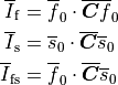
and parameters
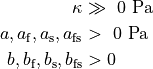
The default parameters are
| a | b | a_f | b_f | a_s | b_s | a_fs | b_fs | kappa | Data |
|---|---|---|---|---|---|---|---|---|---|
| 0.345 | 9.242 | 18.54 | 15.97 | 2.564 | 10.45 | 0.417 | 11.60 | 1000 | Dog |
Guccione et al. myocardial model
The passive behavior of myocardial tissue is modeled by a
nearly-incompressible, transversely isotropic Fung-type constitutive law,
first described by Guccione1991Passive and later also by
Costa1996Three.
The layered organization of myocytes and collagen fibers in the myocardium is
characterized by a right-handed orthonormal set of basis vectors consisting of
the fiber axis , which coincides with the orientation of the
myocytes, the sheet axis and the sheet-normal axis
.
The strain-energy function is given by
![\Psi(\boldsymbol{C})
= \frac{\kappa}{2} \left( \log\,J \right)^2
+ \frac{a}{2}\left[\exp(\overline{Q})-1\right],](../_images/math/f91da6901a55a8ab912cc986ebb62b9d64b062fe.png)
where

and

with 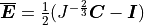 the modified isochoric Green–Lagrange strain tensor.
The bulk modulus
the modified isochoric Green–Lagrange strain tensor.
The bulk modulus  serves as a penalty parameter to
enforce nearly incompressibility and
serves as a penalty parameter to
enforce nearly incompressibility and  is a stress-like scaling
parameter. All other parameters
is a stress-like scaling
parameter. All other parameters 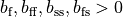 are dimensionless and negative values are not physically
acceptable. Default parameters are:
are dimensionless and negative values are not physically
acceptable. Default parameters are:
| a | b_ff | b_ss | b_nn | b_fs | b_fn | b_ns | kappa | Data |
|---|---|---|---|---|---|---|---|---|
| 0.876 | 18.48 | 3.58 | 3.58 | 3.58 | 1.627 | 1.627 | 1000 | Dog |
and were fitted to produce epicardial strains that were measured previously in the potassium-arrested dog heart.
Several modifications of the original model were published, most notably the simplified version due to Omens1993Measurement and Guccione1995Finite

This is also the version that is implemented in CARP. The parameters are then reduced to:
| a | b_ff | b_ss | b_fs | kappa | Data |
|---|---|---|---|---|---|
| 0.876 | 18.48 | 3.58 | 1.627 | 1000 | Dog |
Mechanical Boundary Conditions
The definition of mechanical boundary conditions follows the same basic concept as is used for defining electrical stimuli. First, a region of the mesh is defined, typically a set of surface nodes or faces, to which boundary conditions are applied. Subsequently, the quantity to apply and its time course is defined. These quantities in mechanics simulations are either a scalar pressure (Neummann boundary conditions), or vector displacements (Dirichlet boundary conditions).
The definition of mechanical boundary conditions uses an analog approach to the definition of electrical stimuli.
A complete definition of a mechanical boundary condition comprises two components,
the definition of the boundary (in terms of vertices or surface elements)
and the loading protocol.
Mechanical loading protocols are described as time traces
describing the time course of applied (scalar) pressure in the case of Neumann boundary conditions
or (vectorial) displacements in the case of Dirichlet boundary conditions.
The definition of Neumann and Dirichlet boundary conditions is very similar
with the major difference being the use of the keyword mechanic_nbc[]
for Dirichlet boundaries,
and mechanic_nbc[] for Neumann boundaries.
Geometry definition: Boundary geometries can be defined in two ways, indirectly by specifying a volume within which all mesh nodes are considered then to be part of this boundary, or, explicitly, by providing a surface file containing all surface elements spanning the boundary.
The default definition is based on a block by specifying the lower left bottom corner and the lengths of the block along the Cartesian axes.
| field | type | description |
|---|---|---|
| name | String | Identifier for electrode used for output (optional) |
| zd | Float | z-dimension of electrode volume |
| yd | Float | y-dimension of electrode volume |
| xd | Float | x-dimension of electrode volume |
| z0 | Float | lower z-ordinate of electrode volume |
| y0 | Float | lower y-ordinate of electrode volume |
| x0 | Float | lower z-ordinate of electrode volume |
| ctr_def | flag | if set, block limits are [ x0 - xd/2 x0 + xd/2], othewise limits are [ x0 x0 + xd] etc |
Alternatively, other types of region than blocks are available such as spheres, cylinders or, the most general case, list of finite elements. See the definition of tag regions for details. Electrodes can be defined then by assigning the index of a tag region to the geometry field:
| field | type | description |
|---|---|---|
| geometry | int | Index of region pre-defined in tag region array tagreg[] |
An explicit definition of boundary conditions is also possible by providing a file holding the defining mesh entities. Here the formats between Neumann and Dirichlet boundaries is different, see below.
| field | type | description |
|---|---|---|
| vtx_file | String | File holding all nodal indices making up the boundary |
| field | type | description |
|---|---|---|
| surf_file | String | File holding all surface elements making up the boundary |
Neumann Boundary Conditions
The definition of loading protocols differs between Neumann and Dirichlet boundaries due to the different physical quantities applied to the boundaries, i.e. scalar pressures always acting perpendicular to the Neumann boundary and vectorial displacement which can be enforced in any direction.
The Neumann loading protocol is defined based on two components, the time course of the applied load as defined in a trace file, and the magnitude of the load. Splitting of these two components offers the advantage of avoiding the redefinition of time traces for different magnitudes of loads.
Loading protocol definition: In the case of Neumann boundary conditions the time course and magnitude of applied pressures must be defined using the keywords summarized in Tab. 16.
| field | type | description |
|---|---|---|
| pressure | Float | pressure imposed on boundary in [kPa] |
| trace | File | trace file describing the time course of pressure |
Dirichlet Boundary Conditions
Loading protocol definition: In the case of Dirichlet boundary conditions the time course and magnitude of applied displacements must be defined using the keywords summarized in Tab. 16.
| field | type | description |
|---|---|---|
| ux | Float | rate of displacement along x in [ ] ] |
| uy | Float | rate of displacement along y in [] |
| uz | Float | rate of displacement along z in [] |
| ux_file | File | trace file describing time course of displacement ux |
| uy_file | File | trace file describing time course of displacement uy |
| uz_file | File | trace file describing time course of displacement uz |
| apply_ux | Flag | flag whether ux displacements are applied or not |
| apply_uy | Flag | flag whether uy displacements are applied or not |
| apply_uz | Flag | flag whether uz displacements are applied or not |
In the Dirichlet case the definition of repetitive loading is also support. The definition follows analog to the definition of electrical stimulation protocols, re-using the same terminology, that is, a single sequence is referred to as a pulse and the duration of a single sequence is referred to as pacing cycle length or basic cycle length.
| field | type | description |
|---|---|---|
| start | float | time at which Dirichlet loading sequence begins |
| duration | float | duration of entire Dirichlet loading sequence |
| npls | int | number of pulses forming the sequence (default is 1) |
| bcl | float | basic cycle length for repetitive stimulation (npls > 1) |
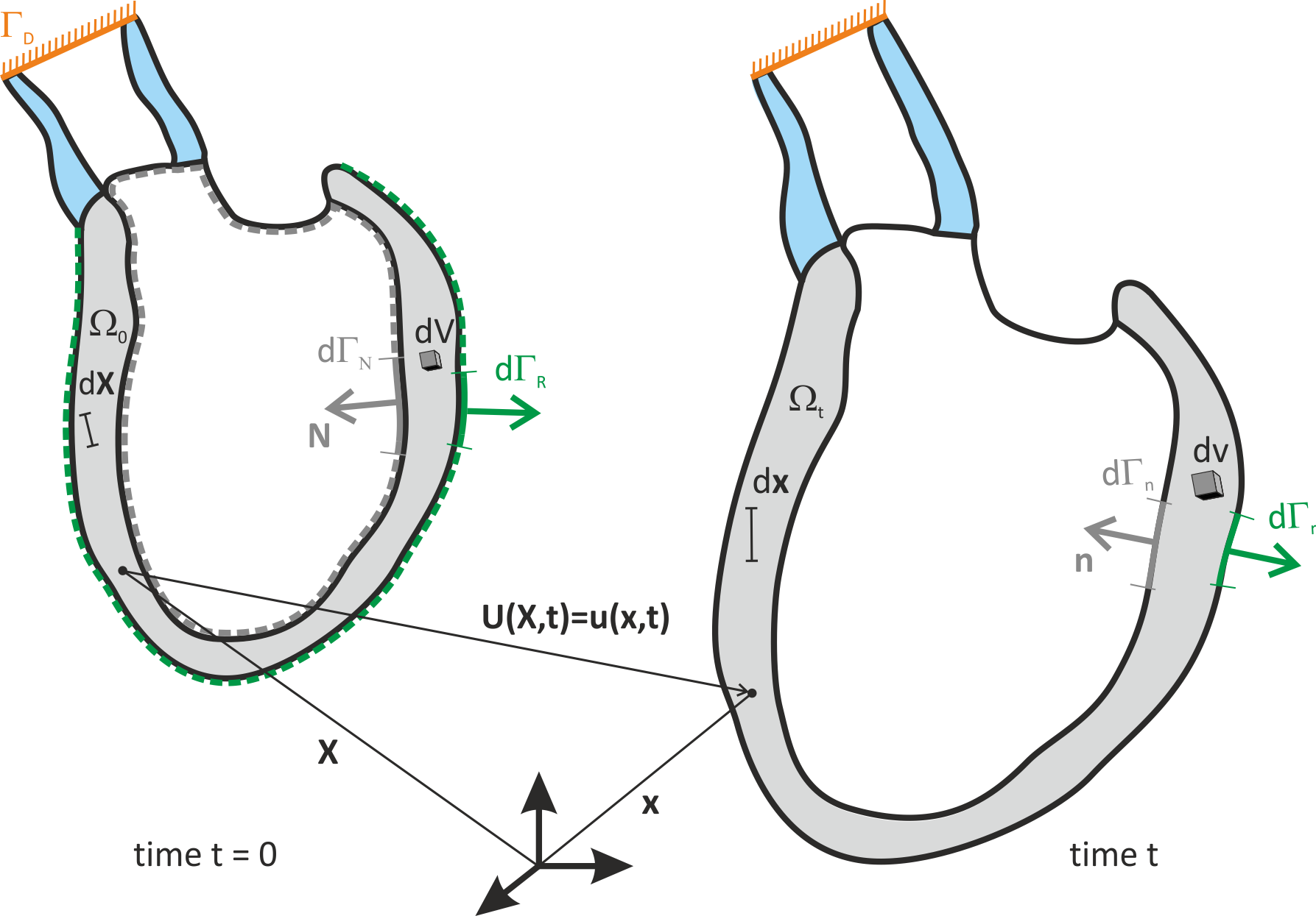
Fig. 53 Deformation of an elastic body  from reference configuration
  to the deformed configuration
  .
Cardiac deformation is constrained by different types of boundary conditions.
At the endocardial surface pressure imposes a Neumann boundary condition.
The larger vessels are elastically anchored in the torso through the mediastinum
which, in general, prevents larger displacements.
Such boundary conditions can be approximated as a homogeneous Dirichlet boundary
or, if image-based motion shall be applied to the model, as an inhomogeneous Dirichlet boundary.
Boundary conditions at the epicardium are more complex due to the presence of the pericardium.
Restraining forces at the epicardium can be approximated as a Robin boundary condition
or, when coupled to a pericardial model, be represented as a mechanical contact problem.
.
Cardiac deformation is constrained by different types of boundary conditions.
At the endocardial surface pressure imposes a Neumann boundary condition.
The larger vessels are elastically anchored in the torso through the mediastinum
which, in general, prevents larger displacements.
Such boundary conditions can be approximated as a homogeneous Dirichlet boundary
or, if image-based motion shall be applied to the model, as an inhomogeneous Dirichlet boundary.
Boundary conditions at the epicardium are more complex due to the presence of the pericardium.
Restraining forces at the epicardium can be approximated as a Robin boundary condition
or, when coupled to a pericardial model, be represented as a mechanical contact problem.
A tutorial on how to apply mechanical boundary conditions in CARPentry simulations is given here.