File Formats

Input File Formats

When setting up a CARP simulation, a node, element and fibre files will generally be required. They must be given the same base name, but different extensions, for example:

meshname.pts
meshname.elem
meshname.lon

To support the quick variation of fiber architecture alternative fiber files can be provided using the orthoname option. In this case meshname is used for nodal and element file, but orthoname is used for the fiber file. For instance, using

-meshname biv_rabbit -orthoname biv_rabbit_hf

would read the following files:

biv_rabbit.pts
biv_rabbit.elem
biv_rabbit_hf.lon

Node file

Extension: .pts

The node (or points) file starts with a single header line with the number of nodes, followed by the coordinate of the nodes, one per line, in $\mu m$ . For example, for a mesh with $n$ nodes we have:

Format	Example
$n$	`10000`
$x_0 \, y_0 \, z_0$	`10.3400 -15.0023 12.023`
$x_1 \, y_1 \, z_1$	`11.4608 -12.0237 11.982`
$\ldots$	$\ldots$
$x_{n-1} \, y_{n-1} \, z_{n-1}$	`-8.4523 36.7472 4.6742`

Element File

Extension: .elem

In general, CARPentry supports various types of elements which can be mixed in a single mesh. However, not all element types are supported in every context, some limitations apply. In electrophysiology simulations element types can be mixed, whereas in mechanics only tetrahedral and hexahedral elements are support. The simple native element file format is as follow

The file begins with a single header line containing the number of elements, followed by one element definition per line. The element definitions are composed by an element type specifier string, the nodes for that element, then optionally an integer specifying the region to which the element belongs.

For example, for a mesh with $n$ elements and where

$T_i$ is the type specifier of element $i$ ,
$N_{i,j}$ indices the $j$ -th node of element $i$ ,
$m_i$ is the number of nodes of element $i$ and
$r_i$ is the optional region of element $i$ ,

the format is given as:

Format	Example
$n$	`20000`
$T_0 \, N_{0,0} \, N_{0,1} \ldots N_{0,m_i-1} \, [r_0]$	`Tt 10 15 123 45 1`
$T_1 \, N_{1,0} \, N_{1,1} \ldots N_{1,m_i-1} \, [r_1]$	`Pr 45 36 100 54 35 74 0`
$\ldots$	$\ldots$
$T_{n-1} \, N_{n-1,0} \, N_{n-1,1} \ldots N_{n-1,m_i-1} \, [r_{n-1}]$	`Tt 9374 7432 1234 4532 1`

The node indicies are determined by their order in the points file. Note that the nodes are 0-indexed, as indicated in Sec. Node file above. The element formats supported in CARP, including their element type specifier strings are given in table Element types supported in CARPentry for different physics. Electrophysiology (EP), Mechanics (MECH) and Fluid (FL). *: for internal use only, not supported in mesh files.. The ordering of nodes in each of the 3D element types is shown in Nodal ordering of 3D element types.

Tab. 3 Element types supported in CARPentry for different physics. Electrophysiology (EP), Mechanics (MECH) and Fluid (FL). ^*: for internal use only, not supported in mesh files.
Type Specifier	Description	Interpolation	#Nodes	Supported in
Ln	Line	linear	2	EP
cH ^*	Line	cubic	2	HPS
Tr	Triangle	linear	3	EP
Qd	Quadrilateral	Ansatz	4	EP
Tt	Tetrahedron	linear	4	EP, MECH, FL
Py	Pyramid	Ansatz	5	EP
Pr	Prism	Ansatz	6	EP
Hx	Hexahedron	Ansatz	8	EP

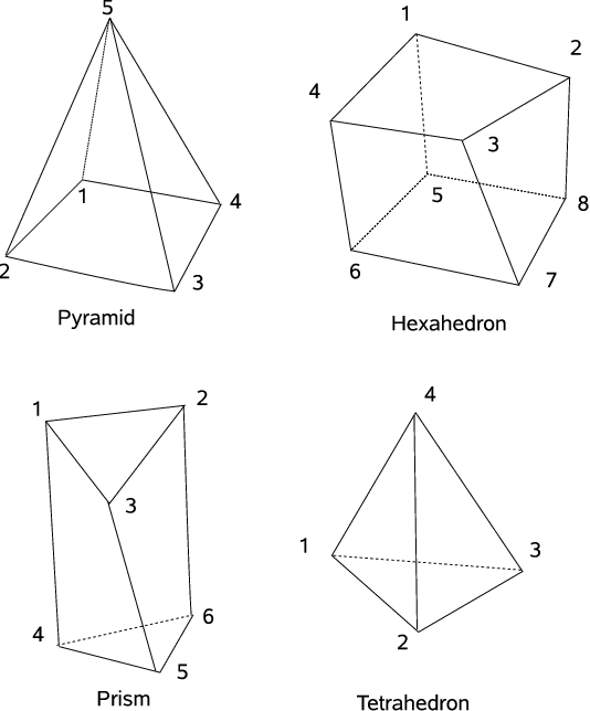
Fig. 6 Nodal ordering of 3D element types

Fiber file

Extension: .lon

Fibres are defined in CARP on a per-element basis. They may be defined by just the fibre direction, in which case a traversely isotropic conductivity or mechanics material model must be used, or additionally specifying the sheet (or transverse) direction to allow full orthotropy in the model.

The file format starts with a single header line with the number of fibre vectors defined in the file (1 for fibre direction only, 2 for fibre and sheet directions), and then one line per element with the values of the fibre vector(s). Note that the number of fibres must equal the number of elements read from the element file.

For example, where $n_f$ is the number of fibre vectors (1 or 2), $f_i,\{x,y,z\}$ are the components of the fibre vector for element $i$ and $s_i,\{x,y,z\}$ are the components of the sheet vector for element $i$ :

Format	Example
$n_f$	`2`
$f_{0,x} \, f_{0,y} f_{0,z} \, [s_{0,x} \, s_{0,y} s_{0,z}]$	`0.831 0.549 0.077 0.473 -0.775 0.417`
$f_{1,x} \, f_{1,y} f_{1,z} \, [s_{1,x} \, s_{1,y} s_{1,z}]$	`0.647 0.026 0.761 -0.678 0.475 0.560`
$\ldots$	$\ldots$
$f_{n-1,x} \, f_{n-1,y} \, f_{n-1,z} \, [s_{n-1,x} \, s_{n-1,y} \, s_{n-1,z}]$	`0.552 0.193 0.810 -0.806 0.369 0.462`

The fibre and sheet vectors should be orthogonal and of unit length.

Vertex file

Extension: .vtx

An collection of preferably unique mesh indices may be stored in a vertex file.

Format	Example
N # number of nodes	192
intra\|extra # definition domain	intra
node_0	47
node_1	123
$\ldots$	$\ldots$
node_N-1	23943

Note

A stimulus electrode file, e.g. apex.vtx may be added in the parameter file as follows:

-stimulus[0].vtx_file apex
The extra-domain refers to the entire user-specified mesh.
The intra-domain refers to the geometry where non-zero fibers were defined.
Although intra and extra should be the the same for tissue-only geometries, CARPentry/mechanics may not like vtx-files stating the vertices as intra domain.

Purkinje file

Extension: .pkje

The format of the Purkinje file is very specific and must be followed carefully. The # character begins a comment. It and everything following on a line are ignored. Section purk-file-rules gives the exact rules for defining Purkinje networks. Below there are comments explaining the different fields inside the file Purkinje.pkje.

Number_of_Cables
Cable 0
Father1 Father2
Son1 Son2
Nodes_Cable
Size
Gap_junction_resistance
Intracellular_conductivity
Node1_x Node1_y Node1_z
...
NodeN_x NodeN_y NodeN_z
Cable 1
...

Note that if a parent or son is unassigned, it is Father2 or Son2 that is assigned a value of -1. An example of a few lines from a Purkinje file follows:

    # Number of Cables present in the tree [0-96]
Cable 0 # Cable 0 is always the first
-1 -1   # no Fathers for Cable 0
2     # Son 1 and Son 2
     # Number of nodes in this Cable
    # Relative size of cable (i.e. #parallel fibres or cross-sectional area)
0   # gap junction resistance (kOhm)
0006  # conductivity (Ohm-cm)
-3400 2200 # NODE 1
-3300 2178 # NODE 2
-3201 2165 # NODE 3
-3090 2154 # NODE 4
Cable 1 # Cable 1, (order must be followed)
-1    # FATHER1 = Cable 0, no Father2
-1    # SON1 = Cable 3, no Son2
    # Number of nodes = 80
0
0
0006
-3090 2154
-3020 2143
-2975 2133
.
.
.

Hint

missing link target purk-file-rules

Purkinje-myocardial junction (PMJ) tuning file

Extension: .pmj

After the global PMJ parameters are applied, individual junction parameters are set based on values in a file. Cables specified must have a PMJ.

#junctions
cable_no R_PMJ PMJ_scale
cable_no R_PMJ PMJ_scale
    .
    .
    .
cable_no R_PMJ PMJ_scale

Pulse file

Note that time values must increase, that is, $t_0 < t_1 < \ldots < t_i < \ldots < t_{N-1}$

N # Number_of_samples
t0  val0
t1  val1
.
.
.
t(N-1)  val(N-1)

Vertex adjustment file

Extension: .adj

N           # Number_of_nodes
intra|extra # definition domain
node_0 val_0
node_1 val_1
.
.
.
node_n-1 val_n-1

Neumann boundary file

Extension: .neubc

TBA

Restitution protocol definition file

Output File Formats

IGB file

Extension: .igb

CARP simulations usually export data to a binary format called IGB. IGB is a format developed at the University of Montreal and originally used for visualizing regularly spaced data. An IGB file is composed of a 1024-byte long header followed by binary data which is terminated by the ASCII form feed character (^L / character 12). For unstructured grids, the individual dimensions are meaningless but x $\\times$ y` $\\times$ z should be equal to the number of vertices. The header is composed of strings of the following format, separated by white space: KeyWord:value Note that the header must be padded to 1024 bytes. The first block of key words in IGB keywords need to be specified. The rest are optional.

Tab. 4 IGB keywords
KeyWord	Type	Description
x	int	number of samples in x
y	int	number of samples in y
z	int	number of samples in z
t	int	number of samples in t
systeme	string	big_endian or little_endian
type	string	binary data type: byte, char, short, long, float, double, int, uint, vec3f, vec4f, vec3d, vec4d
unites	string	units of data
facteur	float	scaling factor for data
zero	float	data zero: true value = IGB_data facteur + zero
org_x	float	lower right x coordinate
org_y	float	lower right y coordinate
org_z	float	lower right z coordinate
org_t	float	time of first slice
inc_x	float	distance between x samples
inc_y	float	distance between y samples
inc_z	float	distance between z samples
inc_t	float	time between samples
dim_x	float	extent in x
dim_y	float	extent in y
dim_z	float	extent in z
dim_t	float	duration
unites_x	string	units of measure for spatial x dimension
unites_y	string	units of measure for spatial y dimension
unites_z	string	units of measure for spatial z dimension
unites_t	string	units of measure for time
comment	string	arbitrary comment
aut_name	string	author’s name
transparent	hex	value for no data

Dynamic Points

Extension: .dynpts

Points may also move in space as functions of time. This is often associated with displacement during contraction, for example. The number of points must remain constant for all time instances, as well as the elements defined by them. Dynamic point files use the IGB format (see IGB file) with data type vec3f.

Vector data file

Extension: .vec and .vpts

To display vector data, an auxiliary set of points must be defined by a file with the .vpts suffix. It follows the same format as the Node file. A file with the same base name but having the extension .vec defines the vector and scalar data. It has the following format:

Format
`data.x` `data.y` `data.z` `[scalar_datum]`
`data.x` `data.y` `data.z` `[scalar_datum]`
$\ldots$
`data.x` `data.y` `data.z` `[scalar_datum]`

The scalar datum, as indicated, is optional. The .vec format can also be used for visualization of fiber orientations stored in .lon files. For this sake, a .vpts file must be generated holding the coordinates of the centers of each element in the mesh. This is conveniently achieved with GlElemCenters and changing the fiber file extension to .vec. For example, for a mesh with $n$ elements and where $f_{i,\{x,y,z\}}$ corresponds to the components of the fiber vector $i$ :

Format	Example
$f_{0,x} \, f_{0,y} f_{0,z}$	`8.12453e-01 -2.22623e-01 1.25001e00`
$f_{1,x} \, f_{1,y} f_{1,z}$	`5.68533e-01 -1.81807e-01 1.04956e00`
$\ldots$	$\ldots$
$f_{n-1,x} \, f_{n-1,y} \, f_{n-1,z}$	`5.70671e-01 -1.67572e-01 1.06615e00`

Vector data can also be input as an IGB file using the types vec3f, vec4f, vec3d, vec4d where 3 or 4 refers to the number of elements in each datum, and d and f refer to float or double. The first 3 elements define the value of the vector field, and the optional 4-th element is the scalar component as above. This file has the suffix .vec.igb.

Auxiliary Grid

Extensions: .pts_t, .elem_t, .dat_t

This format is used by Meshalyzer to display additional data on an auxiliary grid. The grid may contain any of the elements forming the main grid (points,lines,surface elements,volume elements), and the elements may change as a function of time. If scalar data has already been read in, the number of time instances in the auxiliary grid must either be one, or the same as the scalar data. The points file may have only one time instance, which is then assumed constant over all time.

A vertex file is mandatory and has the extension .pts_t. An element file is optional. If present, it has the same base name as the vertex file but with the extension .elem_t. Scalar data may also be optionally defined on the auxiliary grid. The file has the same basename as the vertex file but with the extension .dat_t. The file formats follow:

Tab. 5 Auxiliary data format
.pts_t			.elem_t	.dat_t
.pts_t			.elem_t	.dat_t
#times			#times	#times
#points_time0			#elements_time0	#data_time0
pt(0,0).x	pt(0,0).y	pt(0,0).z	element(0,0)	data(0,0)
pt(1,0).x	pt(1,0).y	pt(1,0).z	element(1,0)	data(1,0)
.	.	.	.	.
.	.	.	.	.
.	.	.	.	.
.	.	.	element(M,0)	.
.	.	.	#elements_time1	.
.	.	.	element(0,1)	.
.	.	.	element(1,1)	.
.	.	.	.	.
pt(N,0).x	pt(N,0).y	pt(N,0).z	.	data(N,0)
#points_time1			.	#data_time1
pt(0,1).x	pt(0,1).y	pt(0,1).z	.	data(0,1)
pt(1,1).x	pt(1,1).y	pt(1,1).z	.	data(1,1)
.	.	.	.	.
.	.	.	element(M,1)	.
.	.	.	#elements_time2	.
.	.	.	element(0,2)	.
.	.	.	.	.