Mechanical Boundary Conditions
Module: tutorials.04_EM_tissue.01_boundary_conditions.run
Section author: Christoph Augustin <christoph.augustin@medunigraz.at> andMatthias Gsell <matthias.gsell@medunigraz.at>
This tutorial demonstrates the time-dependent application of different boundary condition types, i.e., Dirichlet and Neumann boundary conditions, on a cuboidal geometry. For more details on the definition of mechanical boundary conditions in carpentry see manual section mechanical boundary conditions.
Geometry and Material Definition
A simple tetrahedral finite element mesh of a cube shown in Fig. 128 with side length  mm and resolution
  mm as default is generated. The cube is assigned a neo-Hookean material model with shear modulus
  kPa and penalty parameter
  kPa.
kPa.
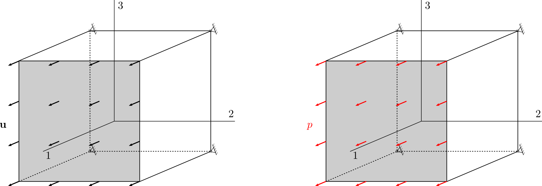
Fig. 128 Schematic representation of the cuboidal geometry including Dirichlet (left panel) and Neumann (right panel) boundary conditions subsequently introduced in Experiment I and Experiment II, respectively.
Boundary Condition Application
For the experiments I & II, movement of nodes located at  is restricted in all directions, i.e., homogeneous Dirichlet boundary conditions are applied (see left and right panels in Fig. 128).
Experiment I - Dirichlet Boundary Conditions
Experiment I provides guidance on the consistent application of inhomogeneous Dirichlet boundary conditions (see left panel in Fig. 128). Nodes located at  are translated under application of displacement
 ![\mathbf{u} = [u_{1},0,0]^{\mathrm{T}}](../../_images/math/89e2bab1597adfe3e8c80985999d384a85262bf8.png) utilizing the command line
utilizing the command line
./run.py --experiment dirichlet --sidelength 1.00 --resolution 0.10 --magnitude 0.10 --visualize
where the parameter experiment selects the correct boundary condition type, parameters sidelength and resolution provide an optional input for the mesh generation and magnitude defines the displacement  in mm. The application of inhomogeneous Dirichlet boundary conditions is time-dependent and necessitates existence of a specific trace file (.trc), in which the time course for the selected displacement is provided calculated as
 ![\mathbf{u} = \phi \mathbf{u}^{\mathrm{s}} = \phi [u_{1}^{\mathrm{s}},u_{2}^{\mathrm{s}},u_{3}^{\mathrm{s}}]^{\mathrm{T}}](../../_images/math/5632f5a7fa421a64b242cf46c51b86b18aaa166a.png) , where
, where  represents the scale factor (see Fig. 129).
Note
Node selection for application of Dirichlet boundary conditions is currently based on internal functions, but can alternatively be performed utilizing a vertex file (.vtx).
Experiment II - Neumann Boundary Conditions
Experiment II provides guidance on the consistent application of Neumann boundary conditions (see right panel in Fig. 128). Nodes located at are translated under application of pressure  on the corresponding surface triangles utilizing the command line
./run.py --experiment neumann --sidelength 1.00 --resolution 0.10 --magnitude 5.00 --visualize
where the parameter experiment selects the correct boundary condition type, parameters sidelength and resolution provide an optional input for the mesh generation and magnitude defines the applied pressure in kPa. Again, the application of Neumann boundary conditions is time-dependent and necessitates existence of a specific trace file (.trc), in which the time course for the selected pressure is provided calculated as  , where represents the scale factor (see Fig. 129).
Note
Element selection for application of Neumann boundary conditions is currently based on internal fuctions, but can alternatively be performed utilizing a surface element file (.neubc).
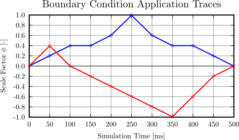
Fig. 129 Dirichlet (blue) and Neumann (red) boundary condition application traces indicating the time-dependent application using a scale factor during simulation specified in corresponding trace files (.trc).
Experimental Results
Upon application of the command lines introduced above, results provided in Fig. 130 will be obtained. While in Experiment I inhomogeneous Dirichlet boundary conditions are consistently stretching the cube, Neumann boundary conditions in Experiment II administer both, compression and tension on the cube (compare boundary condition application traces in Fig. 129).
Fig. 130 Results obtained upon application of command lines introduced in Experiment I using Dirichlet boundary conditions (left panel) and Experiment II using Neumann boundary conditions (right panel) with the color-code representing displacement in  -direction (top row) and
  principal stress (bottom row).
For the experiments III & IV, the plane at is attached to a spring acting in all directions, i.e., homogeneous Robin boundary conditions are applied.
Experiment III - Dirichlet Boundary Conditions
Experiment III provides guidance on the consistent application of inhomogeneous Dirichlet boundary conditions (see left panel in Fig. 128). Nodes located at are translated under application of displacement utilizing the command line
./run.py --experiment dirichlet --fixation weak --sidelength 1.00 --resolution 0.10 --magnitude 0.10 --visualize
where the parameter experiment selects the correct boundary condition type, parameters sidelength and resolution provide an optional input for the mesh generation and magnitude defines the displacement in mm. The application of inhomogeneous Dirichlet boundary conditions is time-dependent and necessitates existence of a specific trace file (.trc), in which the time course for the selected displacement is provided calculated as , where represents the scale factor (see Fig. 129).
Note
Node selection for application of Dirichlet boundary conditions is currently based on internal functions, but can alternatively be performed utilizing a vertex file (.vtx).
Experiment IV - Neumann Boundary Conditions
Experiment IV provides guidance on the consistent application of Neumann boundary conditions (see right panel in Fig. 128). Nodes located at are translated under application of pressure on the corresponding surface triangles utilizing the command line
./run.py --experiment neumann --fixation weak --sidelength 1.00 --resolution 0.10 --magnitude 5.00 --visualize
where the parameter experiment selects the correct boundary condition type, parameters sidelength and resolution provide an optional input for the mesh generation and magnitude defines the applied pressure in kPa. Again, the application of Neumann boundary conditions is time-dependent and necessitates existence of a specific trace file (.trc), in which the time course for the selected pressure is provided calculated as , where represents the scale factor (see Fig. 129).
Note
Element selection for application of Neumann boundary conditions is currently based on internal fuctions, but can alternatively be performed utilizing a surface element file (.neubc).
Experimental Results
Upon application of the command lines introduced above, results provided in Fig. 131 will be obtained. While in Experiment III inhomogeneous Dirichlet boundary conditions are consistently stretching the cube, Neumann boundary conditions in Experiment IV administer both, compression and tension on the cube (compare boundary condition application traces in Fig. 129).
Fig. 131 Results obtained upon application of command lines introduced in Experiment III using Dirichlet boundary conditions (left panel) and Experiment IV using Neumann boundary conditions (right panel) with the color-code representing displacement in -direction (top row) and principal stress (bottom row).