Basic visualization using meshalyzer
Module: tutorials.visualization.meshalyzer.run
Section author: Edward Vigmond <edward.vigmond@u-bordeaux.fr>
Introduction to meshalyzer
meshalyzer is a visualization tool for CARP, capable of displaying 4D sets on meshes and allowing user interaction to investiagte data. The software can be downloaded from GitHub. meshalyzer needs a mesh and optionally, data to display on the mesh.
Generate Model and Data
First we need something to display. Generate the model and data with
./run.py [--np n] [--bidomain]
Use the bidomain flag if you want to look at extracellular potential data. This may take a while, especially if you have a low core count. This is a one time operation.
Launch meshalyzer
meshalyzer
A file dialog appears from which you can navigate to any subdirectory of meshes and select block.pts.
The meshalyzer windows will pop up automatically. One window is the control window with many widgets for controlling the display. The other window is the model window which displays the data on the model. The model window is white because there are no surfaces in the model and that is the entity displayed by default. Creating surfaces is a one time operation which is done by:
click ``File/Compute surfaces`` from the top menu bar
click the *OK* to write it to disk
Right now, there is no data, so it is one colour, orange. Let’s read in some data. The file selector will be in the directory of the last file selected.
click on File/Read IGB data from the top menu bar
go up 2 directories by clicking .. twice
select the directory meshalyzer_test
select 'vm.igb'
In the model window, the rectangle should be black on a white background. The tissue is black because it is all at rest.
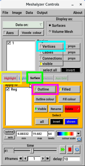
Fig. 172 Meshalyzer control window showing button to toggle vertex display (cyan box), tabs for Highlighting (yellow box) and within the Surface tab (green box), the button to toggle display of the surface element outlines (magenta box).
Advance in time
Put your mouse in the model window. Press the right arrow. Notice how the time advances in the control window. However, you still do not see anything change. This is because the colour scale is optimized for the first frame of data. To reoptimize the colour scale for a particular frame, put the mouse in the model window and press o. The stimulus was applied at 2 ms so make sure you advance at least that far. You can go backwards in time with the left arrow.
The time instant displayed can also be controlled with the time slider. Clicking to the left or right changes decrements or increments the time respectively, while the time button can be dragged while holding the middle mouse button
Watch a movie
In the control window, press the double arrow. The time will advance until the last frame. The animation can be stopped with the pause button.
To make a movie, click on Output/PNG sequence from the top menu bar in the control window. A series of PNGs will be created which are numercially ordered so you can use software like ffmpeg to create a movie. You will be asked for the base name of the files on to which will be appended a number. The movie starts from the frame displayed so make sure you are not at the last frame. The time can be controlled with the time slider at the bottm of the control window.
Inspecting a single node
Click on the Highlight tab in the Control widget.
Now turn on highlighting by clicking On.
Let’s select a node near the middle of the sheet. Before you can select a point, you need to be able to see the points. There are 2 ways to do this
- turn on point display by clicking on the
Verticesbutton in the control window - click on the
Surface taband display theOutline
Click on Pick Vertex in the Highlight tab (it should turn red) and try to pick a point near the center of the sheet using mouse button 1.
If you successfully picked a point, it will be a red dot and the attached surface elements will be outlined in gold and filled in with pink.
The vertex field will be updated in the Highlight tab. If nothing was picked or you want to select another point, you can also press the p key with the mouse in the model window (the button turns red as well in the control window) and try again. Sometimes, zooming in helps.
Note
To zoom, drag while holding mouse button 3. To translate the model, hold mouse button 2. Rotate with mouse button 1. For those without 3 button mice, you can also hold the shift and control keys while depressing the mouse button.
Tip
If your control window gets buried or you lose track of it, just press C in the model window.
Conversely, from the control window, select Image/Raise Window from the top menu bar to raise the model window.
Highlighting
Once you have selected your point, you can turn off the outline or points. Looking at the Highlight tab, you can see the element selected its data value at that particular point in time. To find out more information, click on the gold ? button. This opens the highlight window. The top line indicates the vertex highlighted and how many vertices are in the model. The third line tells you the coordinates of the selected point. Below, there is also the connectivity information showing all elements of which the node is a part, as well as all nodes which are connected by an edge. These items are clickable and become highlighted themselves.
Select an attached surface element from the list in the highlight window.
You will see a blue outline and scrolling down in the window you will see the information about the surace element. All highlighted items hve a gray background in the list. Now, let’s see data as a function of time.
Click on Time Series in the Highlight tab.
A window will pop up with the time trace at that node. The vertical green line indicates the current time. Put the cursor on the time slider and scroll it while holding the middle mouse button.The green line will move.
Tip
Clicking the middle mouse button in the time series window will show the coordinates of the mouse.
Comparing nodes
Suppose we want to compare the time series at two nodes. First, we need to store the visible time trace.
Click on the
Holdbutton at the bottom of the time trace window.Put the mouse in the
Vertexinput field and change the highlighted node by- rolling the mouse wheel
- dragging the mouse while clicking
- typing a new number
- repicking as above
You will see the red time trace update to the new node highlighted and the original trace is blue. Several traces may be stored.
If you want to save the curves to disk, click the Write button, select a name, and an ASCII file will be written. When you want to get rid of the curves, put your mouse on the time trace and press mouse button 3, which pops up a menu from which you select clear static curves.
Saving the State
Adjust the display to something that you like. You can adjust the colour scale, the orientation and scale of the block, and the time displayed. Once you have it perfect, save it:
click on File/Save state from the top menu bar
enter a name, eg., 'testsave'
Now, change the display of the model again, even clearing any static timer series. You would now like to get the old view back,
click on File/Restore state from the top menu bar
select 'testsave.mshz'
It should look the same as before. You should even see the previously held time curves. If you just want to save the current view without any of the properties,
you can Save transform and then Read transform from the File menu.
Different Data Set
If you have run the bidomain simulation, you can load a new data set. We will choose an IGB data set. IGB files are a particular format of data file composed of an ascii header and a binary data. Meshalyzer can also read plain ASCII files with one data value for line for each node.
click on File/Read IGB data from the top menu bar
select 'phie.igb'
go to time frame 6
type o in the model window.
The model window will be mostly white as the model merges with the background.
Tip
You can change the background color under Image/background colour
If you advance the time to almost the end, you will only see a few colours. This is because the data range has changed. The colour scale can be set to optimize every new frame. To do this
click on the auto button on the left side of the colour box below the optimal button.
Now, you will see all colours every frame.
More details on how to use meshalyzer and its capabilities are found in the next tutorial More meshalyzer tricks as well as meshalyzer manual