`Advanced visualization using meshalyzer`

Module: tutorials.visualization.meshalyzer_adv.run

Section author: Edward Vigmond <edward.vigmond@u-bordeaux.fr>

More meshalyzer tricks

While everything is explained in the manual, no one ever wants to RTFM so a few features of meshalyzer are explained here to make life simpler.

Generate Model and Data

First we need something to display. Generate the model and data with

./run.py [--np n] [--bidomain]

Use the bidomain flag if you want to look at extracellular potential data. This may take a while, especially if you have a low core count. This is a one time operation.

Launch meshalyzer

meshalyzer  model data

Model window short cuts

key	action
c	Pops the control window puts it in the corner of the model window
o	optimize colour scale
p	select vertex
r	reread the data. Good for monitoring long runs as they happen
->	advance in time one step
<-	go back one time step

Note

For flat surfaces, it is best to turn off lighting. Colours will be darker and more uniform.

Transparency

Surface transparency is enabled by selecting the Fill colour on the Surface tab. Picking an Opacity of less than one will result in transparency. This can be selected on a per surface basis. As part of rendering transparent surfaces, elements are ordered by z, but only within each surface. Thus, if multiple surfaces are being rendered, results may not be as expected. In this case, you may try Images/Reverse draw order to see if the rendering is improved.

Clipping Planes

Bring up the clipping plane dialog: Data/Cliiping
Six planes are available. On the bottom left, click n the clicking plane that you wish to set. The virtual trackball to the immedoiate right should update to the selected clipping plane orientation. The arrow points to the visible side of the plane. To reorient the plane, click and drag the trackball. If you reorient the model in the model window, the trackball will update.
The plane may be translated by dragging the Intercept. The up and down arrows move it 0.01 in the appropriate direction.

Linking

One sometimes would like to compare two simulations, either different conditions on the same mesh or on different meshes. In such cases, it is important to have the exact same vantage, colour scale, time, etc. Synchronization is a way for passing these parameters between an arbitrary number of running meshalyzer instances. To use synchronization

Start up two instances of meshalyzers.

Hint

you can enter all files on the command line starting with the model name. The points file basename may have a trailing “.” so you can use tab-completion easily. For example, if the name of the model is heart.pts, you can invoke meshalyzer heart, meshalyzer heart. or meshalyzer heart.pts.

Open the link dialogue by clicking File/Link
Select the meshlyzer instance that you would like to link from the upper pane and press link selected. The process ID of the instance should move to the lower pane.
If you then open the other instance, you should see that it is now linked to the first.
Change the view (move, rotate, scale) and press v in the model window. Now the linked model will change to match.
Linking an instance to an already linked group will link the new instance to all members of the group. Theoretically, an arbitrary number of meshalyzers can be linked. Open a new instance of meshalyzer and link it to one of the existing meshalyzers.Hit v in any window and see what happens.
Turn on some clipping planes and sync them.

What if the starting oreintations of the models are not the same? For example, maybe the Y and Z axes are swapped between models. To addres this situation, in each model

Image/Reset transform
Image/Sync/Reference view
Rotate one model so that it aligns with the other(s) and in that meshalyzer Image/Sync/Set reference view

Now, manipulate a model view and sync the views. They should correspond. The key presses in the model window are helpful.

key	action
t	sync times
v	sync viewport

Discrete Levels and Isochrones

Sometimes we wish to display a more discrete colour scale and not a continuous range. In this case,

First we need to generate some data. Go to the basic Meshalyzer tutorial and run:
```
run.py --np=4 --monitor=10  --tend 150 --APD=8
```
Advance the time until the wavefront is part way across the slab. Save a PNG version of the image. Examine the metadata of the file with a program like identify or an Exif viewer:
```
identify -verbose image.png
```
You will see information regarding the data file used to create the image, the range of data displayed and number of colour levels, as well as the time frame.
When the simulatiobn has finished, load the activation data set meshalyzer_test/init_acts_vm_act-thresh.dat. Set the min and max colour values to 0 and 40, respectively, and choose a low number of colour levels, eg., 5.
Open the isolines widget under Data. Turn on isolines, change the start and end values and choose the number of lines to be one more than the number of colour levels. The lines and borders shoulmd match up exactly.
Output the colour bar, under Output/Colour Bar. Look at the resulting file with the program eog for example. Note how it has the correct number of levels. If the colours look different, it is due to lighting effects.
Going back to the isochrones, datify the isolines and save them. Change the dataset back to vm.igb.
File/Read Aux Grid and find isoLines.pts_t. In the Aux Grid tab, datify the lines and adjust the colour scale.

Branch Cuts

The rotational angle $\phi$ is an example of a variable which wraps around so that 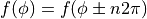$f(\phi)=f(\phi\pm n 2\pi)$ for any integrer n. In this case, a branch cut is made at $-\pi$ to restrict $\phi$ to the range $[-\pi,\pi)$ . We cannot interpolate across the branch cut or we get nonsense, that is, if we simply average $-\pi$ and $\pi$ , we get 0 instead of $\pi$ . Meshalyzer is branch cut aware.

Load the canine mesh with the $\phi$ coordinate (see Applying UVCs but take the 3rd field of dog_vtx.pts ):
```
meshalyzer canine dog_phi.dat
```
Display the zero isoline without a branch cut. Note how the line crosses the whole heart, even the $-\pi$ region, which is spurious.
Turn on the branch cut: Data/Branch cut/[-pi,pi) and see the proper isovalue line.

Ignoring some data values

Sometimes data sets may contain spurious values, where a computation fails. An example of this is a map of activation times when propagation fails in part of the tissue. In this case, we define a dead range of data which will not be displayed.

Select Data/Dead range
Activate the functionality by clicking Dead data
To ignore NaN’s (IEEE not-a-number), click on the button
Define the range of permissible values which may be open ended.
Select the colour (or lack thereof) to display these elements.
Apply the changes.

More details on how to use meshalyzer and its capabilities are found in the meshalyzer manual