`Ring`

Module: tutorials.04_EM_tissue.08_ring.run

Section author: Christoph Augustin <christoph.augustin@medunigraz.at> and Matthias Gsell <matthias.gsell@medunigraz.at>

This example provides pure mechanics and electromechanics examples on a simple ring geometry.

Problem Setup

This problem generates a simple ring mesh using the carputils.mesh.Ring class. The ring is tessellated into tetrahedra as shown below:

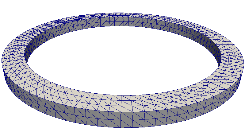
Fig. 144 Automatically generated (CGAL-based) mesh of a LV ring model.

In all experiment types in this example, the top and bottom surfaces of the ring are constrained to lie in the same plane with Dirichlet boundary conditions, and an additional three nodes on the bottom ( $z=0$ ) surface are constrained such that free body rotation and translation is prevented. Two nodes on the x axis are prevented from moving in the y direction, and one node on the y axis is prevented from moving in the x direction:

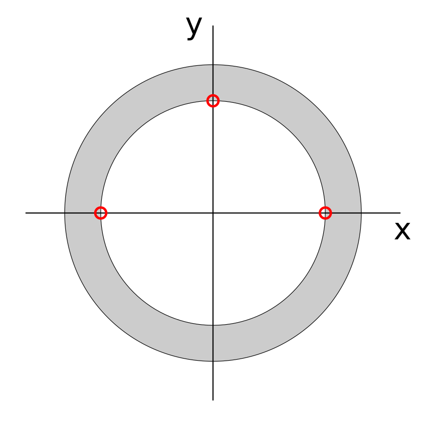
Fig. 145 Additional boundary conditions applied to prevent rigid body motion.

Experiments

Three types of experiments are defined:

active-free - Run an active contraction simulation without constraints on cavity size or pressure. This corresponds to a Langendorff-setup where the LV cavity is not pressurized.
active-iso - Run an active contraction simulation with an isovolumetric cavity constraint. The LV cavity volume is kept constant, that is, both inflow and outflow valves are closed.
active-pv-loop - Run an active contraction simulation with circulatory coupling. In this case the LV ring is coupled with a simple LA model (constant pressure) and a 3-element Windkessel model through inflow and outflow valves to regulate preload and afterload. The inflow valve closes when the LV pressure exceeds a prescribed pressure (approximately the pressure in the LA at end diastole). The outflow valve opens when the LV pressure exceeds the input pressure of the attached Windkessel model and closes when outflow turns negative. A lumped representation of this setup is given in Fig. 146.

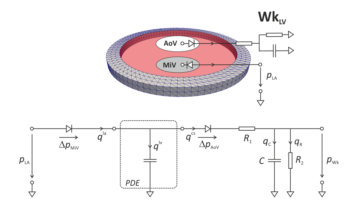
../../_images/ring_circulatory_coupling.png

Fig. 146 Lumped representation of the PDE ring model coupled to simplified model of the circulation. A prescribed pressure in the left atrium, $p_{\mathrm{LA}}$ serves to steer preload and a 3-element Windkessel model serves as afterload model. The valves are modeled as simple resistors to allow pressure gradients to build up.

Other Arguments

Another key argument is the stress model. The available active stress model is:

TanhStress - A simple stress model based on Niederer et al. (2011). Cardiovascular research, 89(2), 336-343. (see TanhStress model for details).

The stress model can be modified with the following arguments:

s_peak - Peak stress in kPa (default: 100 kPa)
tau_c - Time constant governing rate of rise in active stress model (default: 10 ms)

Usage

To run a simple active-free-experiment call

./run.py \
--experiment active-free  `# experiment to run, possible choices: \
                           #     'active-free', 'active-iso' or 'active-pv-loop'` \
--duration 500            `# duration of the experiment (default 500 ms)` \
--s_peak 100              `# Peak stress in kPa (default 100 kPa)` \
--tau_c 10                `# Time constant governing rate of rise \
                           #     in active stress model (default 10 ms)` \
--np 10                   `# number of processes` \
--visualize               `# visualize with meshalyzer`

or call

./run.py \
--experiment active-pv-loop  `# possible experiments: \
                              #     'active-free', 'active-iso' or 'active-pv-loop'` \
--duration 500               `# duration of the experiment (default 500 ms)` \
--s_peak 100                 `# Peak stress in kPa (default 100 kPa)` \
--tau_c 10                   `# Time constant governing rate of rise \
                              #    in active stress model (default 10 ms)` \
--np 10                      `# number of processes` \
--visualize                  `# visualize with meshalyzer`

for a simple active-pv-loop-experiment.

Expected results

Simulation results computed are shown in the following for a full heartbeat.

Fig. 147 Shown is the fiber projected strain on the left (blue: -0.15, red: 0.22) and active tension $\sigma_{\rm a}(\mathbf{x},t)$ on the right (blue: 0.0 kPa, red: 90 kPa).

Post-processing

The active-pv-loop-experiments output a cavity-information file (usually called cav.LV.csv) which contains pressure information, volume information, flow rates and many other additional informations. This cavity-information file can be used for a post-processing analysis using the following tools.

cavplot

The cavplot-tool is a simple tool for plotting the pressure volume relation. Call

cavplot cav.LV.csv

to plot the pressure-volume-relation, see figure Fig. 153. To plot just a single trace use the --mode flag and one of the options combined, pvloop, volume, pressure, flux, pressuredot, fluxdot, q_out, q_in. If you want to add the loading phase to your plot use the --loading flag.

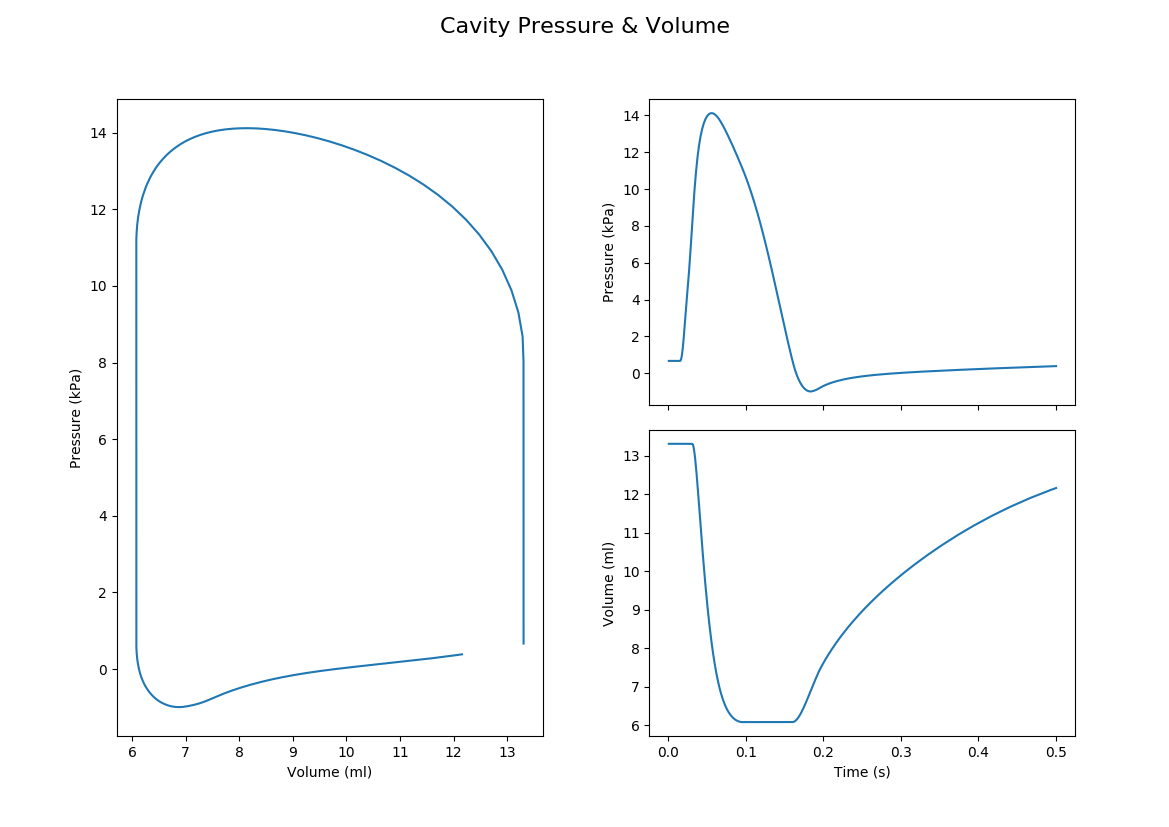
Fig. 148 Pressure-volume plot produced by cavplot.

cavinfo

The cavinfo-tool is an improved version of the cavplot tool. In addition to plotting pressure-volume data cavinfo performs a detailed analysis, computes various metrics and annotates the pressure-volume plots. Call

cavinfo --file cav.LV.csv     `# cavity information file` \
        --output cavity.info  `# output file name (default 'cavity.info')`

to plot the pressure-volume-relation and to determine many other quantities as ESV, EDV, etc., see figure Fig. 154. All the information is stored in the output file and printed to the terminal, see output below.

cavity file         : cav.LV.csv
negative flow       : True
time range          : 0.000 - 500.000 ms
IVC begin           : 17.000 ms
ejection begin      : 32.000
IVR begin           : 101.000 ms
V0                  : 9.792 ml
EDV                 : 13.286 ml  ( at 32.000 ms )
ESV                 : 6.080 ml  ( at 100.000 ms )
SV                  : 7.206 ml
EF                  : 54.238 %
peak flow           : 0.268 ml/ms  ( 268.131 ml/s ) ( 0.268 L/s )  ( 16.088 L/min )
peak flow time      : 41.000 ms
open pressure       : 8.680 kPa  ( 65.109 mmHg )
open pressure time  : 32.000 ms
peak pressure       : 14.119 kPa  ( 105.902 mmHg )
peak pressure time  : 56.000 ms
mean pressure       : 13.022 kPa  ( during ejection )
hm peak pressure    : 14.219 kPa  ( 106.651 mmHg )
work                : 93.837 kPa/ml  ( 0.094 J )
estimated work      : 81.394 kPa/ml  ( 0.081 J )
external work       : 94.149 kPa/ml  ( 0.094 J )
contraction time    : 39.000 ms  ( peak pressure time - IVC begin )
Ea                  : 1.480 kPa/ml
Ees(E)              : 0.164 kPa/ml

To get the total argument list run cavinfo --help.

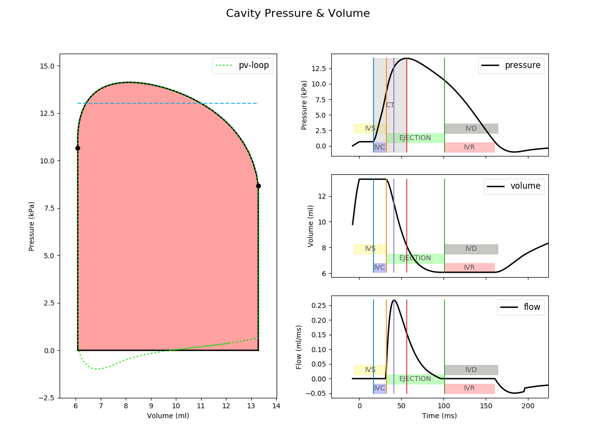
Fig. 149 Pressure-volume plot as produced by cavinfo. Note the additional annotations compared to the plots produced with cavplot shown in Fig. 153.

Hint

The tool is right now part of the pvprocess module but this will be changed!