BiVSlice

Problem Setup

This problem generates a slice bi-ventricular mesh using the carputils.mesh.BiVSlice class. The bi-ventricular slice is tessellated into tetrahedra as shown below:

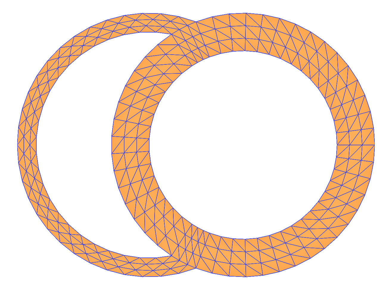
Fig. 150 Automatically generated (CGAL-based) mesh of a LV-RV bi-ventricular slice model.

In all experiment types in this example, the top and bottom surfaces of the slice are constrained to lie in the same plane with Dirichlet boundary conditions, and an additional three nodes on the bottom () surface are constrained such that free body rotation and translation is prevented. Two nodes on the x axis are prevented from moving in the y direction, and one node on the y axis is prevented from moving in the x direction:

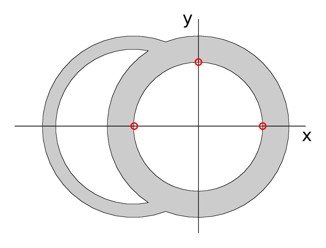
Fig. 151 Dirichlet boundary conditions applied to prevent rigid body motion.

Experiments

Several experiments are defined:

• active-free - Run an active contraction simulation without constraints on cavity size or pressure
• active-iso - Run an active contraction simulation with an isovolumetric cavity constraint
• active-pv-loop - Run an active contraction stimulation with pressure/flux constraints imposed by Windkessel or circulatory models coupled to both RV and LV cavity. In this case both left and right ventricular cavities are coupled to a 3-element Windkessel model

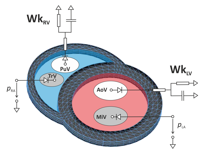
Fig. 152 Lumped representation of the PDE bi-ventricular slice model coupled to a simplified 0D model of the circulation. Prescribed pressure in the left and right atrium serve to steer preload and a 3-element Windkessel model serves as afterload model. The valves are modeled as simple resistors to allow pressure gradients to build up.

Other Arguments

Another key argument is the stress model. The available active stress model is:

• TanhStress - A very simple active stress model based on activation times and constructed with exponential functions which also accounts for length-dependent development of active tension (see TanhStress model for details).

This active stress model is based on

• [1] Niederer et al. (2011). Cardiovascular research, 89(2), 336-343.

The stress model can be modified with the following arguments:

• s_peak - Peak stress in kPa (default: 50 kPa)
• tau_c - Time constant governing rate of rise in active stress model (default: 45 ms)
• ld_on - Turn on length dependence (default: off)

Usage

To run a simple active-free-experiment call

./run.py \
--experiment active-free  `# experiment to run, possible choices: \
                           #     'active-free', 'active-iso' or 'active-pv-loop'` \
--duration 180            `# duration of the experiment (default 180 ms)` \
--s_peak 50               `# Peak stress in kPa (default 50 kPa)` \
--tau_c 45                `# Time constant governing rate of rise \
                           #     in active stress model (default 45 ms)` \
--np 10                   `# number of processes` \
--visualize               `# visualize with meshalyzer`

or call

./run.py \
--experiment active-pv-loop  `# possible experiments: \
                              #     'active-free', 'active-iso' or 'active-pv-loop'` \
--duration 180               `# duration of the experiment (default 180 ms)` \
--s_peak 50                  `# Peak stress in kPa (default 50 kPa)` \
--tau_c 45                   `# Time constant governing rate of rise \
                              #    in active stress model (default 45 ms)` \
--np 10                      `# number of processes` \
--visualize                  `# visualize with meshalyzer`

for a simple active-pv-loop-experiment.

Post-processing

The active-pv-loop-experiments output a cavity-information file (usually called cav.LV.csv) which contains pressure information, volume information, flow rates and many other additional informations. This cavity-information file can be used for a post-processing analysis using the following tools.

cavplot

The cavplot-tool is a simple tool for plotting the pressure volume relation. Call

cavplot cav.LV.csv cav.RV.csv --pressure

to plot the pressure-volume-relation, see figure Fig. 153. To plot just a single trace use the --mode flag and one of the options combined, pvloop, volume, pressure, flux, pressuredot, fluxdot, q_out, q_in. If you want to add the loading phase to your plot use the --loading flag.

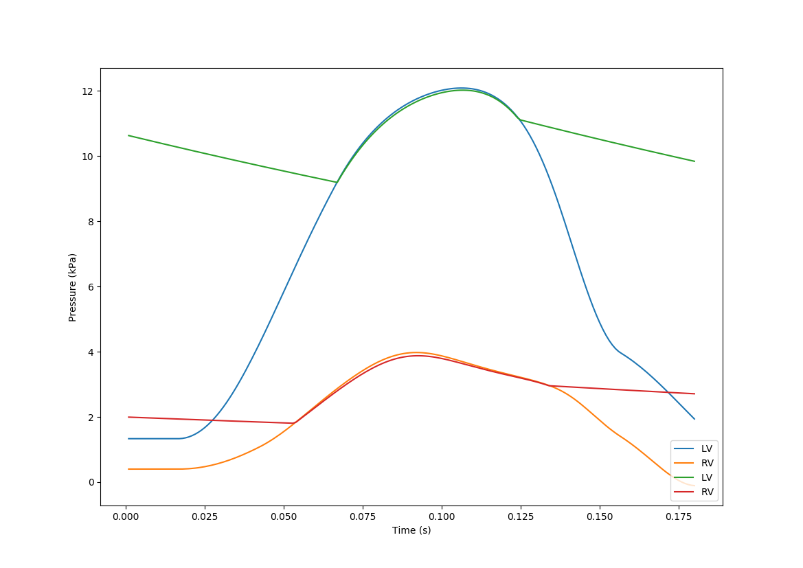
Fig. 153 Pressure plot produced by cavplot. Lines show pressure over time in the left and right ventricle and the pressure in the attached outflow compartments, respectively.

cavinfo

The cavinfo-tool is an improved version of the cavplot tool. In addition to plotting pressure-volume data cavinfo performs a detailed analysis, computes various metrics and annotates the pressure-volume plots. Call

cavinfo --file cav.RV.csv     `# RV cavity information file` \
        --output cavity.info  `# output file name (default 'cavity.info')`

to plot the pressure-volume-relation and to determine many other quantities as ESV, EDV, etc., see figure Fig. 154. All the information is stored in the output file and printed to the terminal, see output below.

cavity file         : 2018-09-13_active-pv-loop_fast_P1-P0_pt_np2/cav.RV.csv
negative flow       : True
time range          : 0.000 - 180.000 ms
IVC begin           : 24.000 ms
ejection begin      : 54.000
IVR begin           : 135.000 ms
V0                  : 5.534 ml
EDV                 : 7.268 ml  ( at 54.000 ms )
ESV                 : 3.503 ml  ( at 134.000 ms )
SV                  : 3.765 ml
EF                  : 51.802 %
peak flow           : 0.083 ml/ms  ( 83.496 ml/s ) ( 0.083 L/s )  ( 5.010 L/min )
peak flow time      : 85.000 ms
open pressure       : 1.849 kPa  ( 13.870 mmHg )
open pressure time  : 54.000 ms
peak pressure       : 3.976 kPa  ( 29.826 mmHg )
peak pressure time  : 92.000 ms
mean pressure       : 3.543 kPa  ( during ejection )
hm peak pressure    : 4.306 kPa  ( 32.296 mmHg )
work                : 13.338 kPa/ml  ( 0.013 J )
estimated work      : 11.977 kPa/ml  ( 0.012 J )
external work       : 13.358 kPa/ml  ( 0.013 J )
contraction time    : 68.000 ms  ( peak pressure time - IVC begin )
Ea                  : 0.788 kPa/ml
Ees(E)              : 0.236 kPa/ml

To get the total argument list run cavinfo --help.

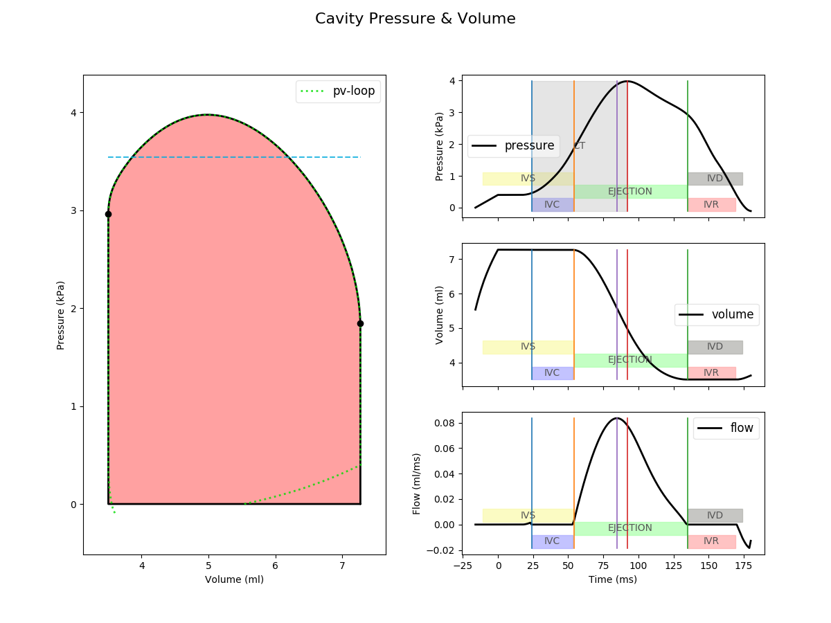
Fig. 154 Pressure-volume plot of the RV as produced by cavinfo. Note the additional annotations compared to the plots produced with cavplot shown in Fig. 153.

Hint

The tool is right now part of the pvprocess module but this will be changed!