`Electro-mechanical coupling`

Module: tutorials.04_EM_tissue.04_EM_coupling.run

Section author: Gernot Plank <gernot.plank@medunigraz.at> and Christoph Augustin <christoph.augustin@medunigraz.at

Electro-mechanical coupling at the tissue scale

This tutorial elucidates the setting up of electro-mechanically coupled tisue simulations. As an example we use a simpliefied model of a left ventricular wedge preparation. For the sake of computational efficiency the apico-basal and circumferential dimension of the wedge are chosen by default to be small and the resolution of the model is coarse. As in the matching single cell stretcher experiment the same EP models (TT2, GPB) and stress models (TanhStress, LandStress, GPB-LandStress-model) are available which cover all three coupling modes (activation-time based ECC, weak calcium-driven ECC and strong calcium-driven ECC). The differences between coupling modes are illustrated in Fig. 52.

Experimental setup

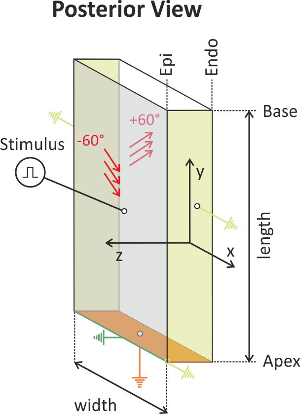
Fig. 138 The setup uses a simple LV wedge preparation where the apicobasal and circumferential dimension can be chosen by setting the --length and --width input parameters. The wedge is mechanically fixated through homogeneous Dirichlet boundary conditions at the apical face of the wedge. At the anterior and posterior faces homogeneous Dirichlet boundary conditions are also applied, preventing any displacement in radial (z-axis) and circumferential (x-axis) direction, but allowing the wedge to slide along the apico-basal (y-axis) direction. Fiber rotation is set to standard values with -60 degrees at the epicardial face and +60 degrees at the endocardial face. The wedge is electrically stimulated epicardially at the center of the preparation.

Input parameters

To run the examples of this tutorial do

cd ${TUTORIALS}/04_EM>_tissue/04_EM_coupling

To inquire the exposed experimental input parameters run

./run.py --help

which yields the following options:

--EP {TT2,GPB}        pick human EP model (default is TT2)

--Stress {LandStress,TanhStress}

                     pick stress model (default is TanhStress)

--width WIDTH        choose circumferential width of wedge in mm

--resolution RESOLUTION

                     choose mesh resolution in mm (default is 2.0 mm)
--duration DURATION  duration of simulation (ms) (default: 500.0 ms)

--mechanics-off      switch off mechanics to generate activation vectors

Expected results

Simulation results computed at a higher spatial resolution of $h=250 \mu m$ are shown in the following for a full contraction-relaxation cycle. Specifically, the activation sequence is shown in terms of all relevant signals involved in active force generation in fig-ecc-wedge.

Fig. 139 Shown are signals involved in the excitation-contraction coupling cascade. A stimulus is delivered at the center of the epicardial surface to initiate the propagation of action potentials. The leftmost panels shows transmebrane voltages $V_{\rm m}(\mathbf{x},t)$ (blue: -90 mV, red: +50 mV). Propagating action potentials initiate Calcium transients which drive the generation of active stress. The mid-left panel shows the intracellular Calcium transients $[Ca_{\rm i}(\mathbf{x},t)$ (blue: 0. $\mu mol$ , red: 1.2 $\mu mol$ ). Due to fiber rotation a significant heterogeneity in fiber stretch, $\lambda$ , is wittnessed, which is shown in the mid-right panel (blue: 0.7, red: 1.3). The rightmost panel shows active tension $\sigma_{\rm a}(\mathbf{x},t)$ (black: 0.0 kPa, red: 40 kPa).

Experiment exp01 (setting up activation-time based tension model)

In a first step we solve only the EP problem with the active stress plug-in enabled to verify that activation sequence and force generation are working properly. Solving of the mechanics problems is turned off by adding the --mechanics-off flag, thus fiber stretch remains constant at $\lambda=1.0$ for the entire simulation. Tension therefore is not modulated by length-dependence. The --visualize option shows transmembrane voltage $V_{\rm m}$ , active stress $\sigma_{\mathrm a}$ and fiber stretch $\lambda$ .

./run.py --EP TT2 --Stress TanhStress --ID exp-em-ti-01 --mechanics-off --visualize

Experiment exp02 (contraction with activation-time based tension model)

Omitting the --mechanics-off flag turns on the computation of deformation. Using the default settings for --length, --width and --resolution leads to a fairly coarse discretization, but allows for sufficiently short simulation cycles. EP in this simulation is driven by a reaction-eikonal approach (see Neic et al [1] for details) which yields undistorted propagation patterns even on coarse meshes. For the sake of saving compute time we use a resolution of 4 mm.

./run.py --EP TT2 --Stress TanhStress --resolution 4 --ID exp-em-ti-02 --visualize

Experiment exp03 (setting up Calcium-driven tension model)

As before in experiment exp01, we solve only the EP problem with the active stress plug-in enabled to verify that activation sequence and force generation are working as expected. As we are using a Calcium-driven active stress model the --visualize option shows also the Calcium signals which serve as input for driving the active stress model.

./run.py --EP TT2 --Stress LandStress --ID exp-em-ti-03 --mechanics-off --visualize

Experiment exp04 (contraction with Calcium-driven tension model)

We repeat experiment exp03 with deformation enabled now. Due to the weak coupling approach used the Calcium signals remain unaltered as compared to experiment exp03 without deformation (i.e. $\lambda=1.0$ ).

./run.py --EP TT2 --Stress LandStress --resolution 4 --ID exp-em-ti-04 --visualize

Experiment exp05 (setting up strongly coupled Calcium-driven tension model)

This experiment repeats exp03, but with strong coupling For the sake of saving compute time only 80 ms activity are simulated to observe the onset of contraction.

./run.py --EP GPB --Stress LandStress --mechanics-off --ID exp-em-ti-05 --visualize

Experiment exp06 (contraction with strongly coupled Calcium-driven tension model)

./run.py --EP GPB --Stress LandStress --resolution 4 --ID exp-em-ti-06 --visualize

Literature

[1]	Neic A, Campos FO, Prassl AJ, Niederer SA, Bishop MJ, Vigmond EJ, Plank G. Efficient compuation of electrograms and ECGs in human whole heart simulations using a reaction-eikonal model. J Comput Phys. 346:191-217, 2017. [Online]