`Tuning velocities and anisotropy ratios`

Module: tutorials.02_EP_tissue.03A_study_prep_tuneCV.run

Section author: Caroline Mendonca Costa <caroline.mendonca_costa@kcl.ac.uk>

Concept

This tutorial introduces the theoretical background for the relationship between conduction velocity and tissue conductivity and how a iterative method to tune the conductivity values to yield a desired velocity for a given setup can be derived. In addition, the definition of anisotropy ratio and its impact on simulation results are presented. A simple strategy to enforce desired anisotropy ratio and conduction velocities is also presented.

Tuning Conduction Velocity

The relationship between conduction velocity and conductivity

A minimum requirement in modeling studies which aim at making case-specific predictions on ventricular electrophysiology is that activation sequences are carefully matched. Conduction velocity in the ventricles is orthotropic and may vary in space, thus profoundly influencing propagation patterns.

As described in Section [Tissue scale], the monodomain model [1] is equivalent to the bidomain model [2] if the monodomain conductivity tensor is given by the harmonic mean tensor, ${\sigma_m}$

(32) $\mathbf{\sigma_m} = (\mathbf{\sigma_i}+\mathbf{\sigma_e})*(\mathbf{\sigma_i}*\mathbf{\sigma_e})^{-1}$

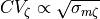
Conduction velocity, CV , is not a parameter in the bidomain equations [2] and as such cannot be directly parametrized. However, assuming a continuously propagating planar wavefront along a given direction, $\zeta$ , one can derive a proportionality relationship [1] between $CV_\zeta$ and $\sigma_{m\zeta}$

(33) $CV_\zeta \propto \sqrt{{\sigma_{m\zeta}}}$

Note

For simplicity, the surface-to-volume ratio, $\beta$ , was ommited in this tutorial, as it is kept constant when tuning conductivities [1]

Conduction velocity as a function of simulation parameters

Experimental measurements of conductivity values are scarce and the variation in measured values across studies is vast. These uncertainties inevitably arise due to the significant degree of biological variation and the substantial errors in the measurement techniques themselves. Modeling and technical uncertainties may also have an impact on model predictions. Particularly, CV depends on the specific model used to describe cellular dynamics, $I_{ion}$ , the spatial discretization, $\Delta_x$ , and on several implementation choices including the time-stepping scheme used, which we represent as $\xi$ . Thus, CV can be represented as a function

(34) $CV_\zeta = CV_\zeta({\sigma_{m\zeta}},I_{ion},\Delta_x,\xi)$

Iterative scheme for conduction velocity tuning

In most practical scenarios, $I_{ion}$ , $\Delta_x$ , and $\xi$ are parameters defined by users in the course of selecting a simulation software, an ionic model and a provided mesh to describe the geometry. Thus, only ${\sigma_{m\zeta}}$ is left which can be tuned to achieve a close match between the pre-specified conduction velocity, $CV_\zeta$ , and the velocity, $\bar{CV_\zeta}$ , predicted by the simulation.

Using (33), and (32) one can find unique monodomain conductivities along all axes $\zeta$ , which yield the prescribed conduction velocities, $CV_\zeta$ , by iteratively refining conductivities based on $\bar{CV_\zeta}$ , measured in simple 1D cable simulations. The iterative update scheme we propose is given as

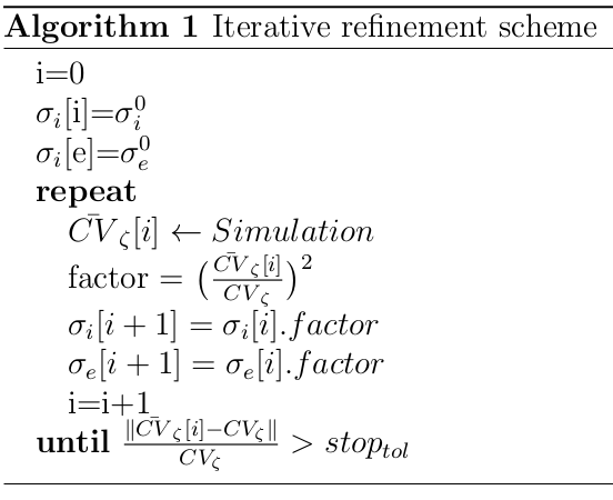
Fig. 63 Iterative update scheme to tune conductivity values based on a prescribed velocity $CV_\zeta$ [1]

The algorithm is implemented as follows. Given an initial conductivity “guess”, ${\sigma_i}^0$ and ${\sigma_e}^0$ and all other simulation parameters defined by $I_{ion}$ , $\Delta_x$ , and $\xi$ , a simulation is run using a 1D cable and the conduction velocity is computed, as described in the figure below:

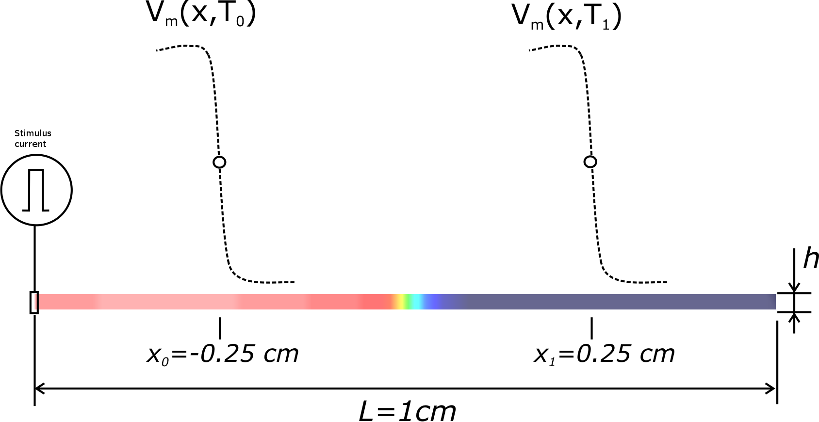
Fig. 64 Setup for convergence testing. A pseudo 1D cable is created, which is in fact a 1 element tick cable of hexahedral elements, where $h$ is the edge length of each hexahedral, which also defines the spatial resolution. Propagation is initiated by applying a transmembrane stimulus current at the left corner. $T_0$ , and $T_1$ correspond to wavefront arrival times recorded at locations $x_0 = -0.25$ cm and $x_1 = 0.25$ cm, respectively. CV is computed as $CV = (x_1 - x_0)/(T_1 - T_0)$ .

Using $factor = (CV_zeta/\bar{CV_zeta})^2$ , the conductivities ${\sigma_i}[i+1]$ and ${\sigma_e}[i+1]$ are updated. A new simulation is then run with the new conductivities. These steps are repeated until the error in CV is below a given tolerance, $stop_{tol}$

Problem Setup

This tutorial will run a simulation on a 1D cable and compute the simulated CV, $\bar{CV}$ , and/or run the iterative scheme shown Figure Fig. 63 to compute the conductivity ${\sigma_m}$ which yields the prescribed CV for the chosen simulation setup.

Usage

The experiment specific options are:

--resolution RESOLUTION
                      Spatial resolution
--velocity VELOCITY   Desired conduction velocity (m/s)
--gi GI               Intracellular conductivity (S/m)
--ge GE               Extracellular conductivity (S/m)
--ts TS               Choose time stepping method. 0: explicit Euler, 1:
                      crank nicolson, 2: second-order time stepping
--dt DT               Integration time step on micro-seconds
--converge {0,1}      0: Measure velocity with given setup or 1: Compute
                      conductivities that yield desired velocity with given
                      setup
--compareTuning       run tuneCV with --resolution 100 200 and 400 with and
                      without tuning and make comparison plot
--compareTimeStepping
                      run tuneCV with --resolution 100 200 and 400 with
                      Explicit Euler and Crank Nicolson and make comparison
                      plot
--compareMassLumping  run tuneCV with --resolution 100 200 and 400 with and
                      without mass lumping and make comparison plot
--compareModelPar     run tuneCV with --resolution 100 200 and 400 with
                      original Ten Tusher cell model and with reduced
                      sodium conductance and make comparison plot
--ar AR               run tuneCV with for CV_f = 0.6 and CV_s = 0.3 m/s with
                      given anisotropy ratio (ar)

The user can either run single experiments, do a comparison of the multiple resolutions with the options --compareTuning, --compareTimeStepping, --compareMassLumping, and --compareModelPar, or compare the change in conductivities with different anisotropy ratios

Run 1D examples

To run the experiments of this tutorial do

cd ${TUTORIALS}/02_EP_tissue/03A__study_prep_tuneCV

compareTuning:

To compute the conductivities for resolutions of 100, 200, and 400 um with and without tuning, run:

./run.py --compareTuning --visualize

After running this command you should see the following plot

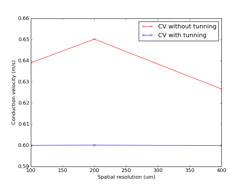
Fig. 65 Simulated CV for different resolutions with and without the iterative tuning scheme.

Note

Notice that CV varies with resolution in a non-linear fashion and CV is constant when the iterative scheme is applied.

compareTimeStepping:

To compare the effect using the Explicit Euler or Crank Nicolson methods for the resolutions of 100, 200, and 400 um run:

./run.py --compareTimeStepping --visualize

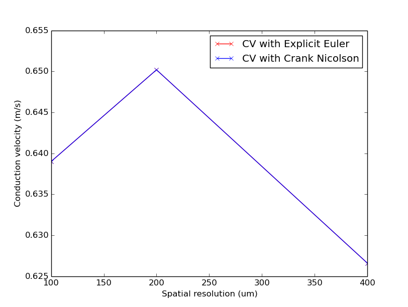
../../_images/tuneCV-compareTimeStepping.png

Fig. 66 Simulated CV for different resolutions with and without the iterative tuning scheme.

Note

Notice that CV varies with resolution virtually identically with both time-stepping schemes.

compareMassLumping:

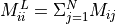
Mass lumping is a common numerical technique in FEM to speed up computation. The mass matrix, $M$ , is made diagonal, implying that its inverse is also diagonal, and solving the system is trivial. The lumped mass matrix, $M^L$ , is computed by setting its main diagonal to be

$M_{ii}^L = \Sigma_{j=1}^N M_{ij}$

To compare the effect of using mass lumping on CV for the resolutions of 100, 200, and 400 um run:

./run.py --compareMassLumping --visualize

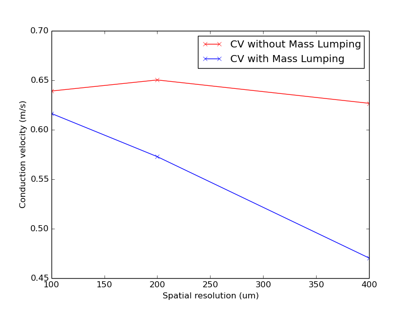
../../_images/tuneCV-compareMassLumping.png

Fig. 67 Simulated CV for different resolutions with and without mass lumping.

Note

Notice that CV varies with resolution in both cases, but the decrease in CV for coarser resolutions is much steeper with mass lumping.

compareModelPar:

To compare the effect of modifying the sodium conduction on CV for the resolutions of 100, 200, and 400 um run:

./run.py --compareModelPar --visualize

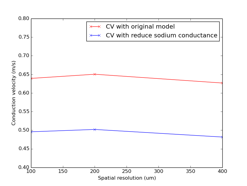
../../_images/tuneCV-compareModelPar.png

Fig. 68 Simulated CV for different resolutions with the original Ten Tusher model and with reduce sodium conductance

Note

Notice that CV varies with resolution similarly in both cases, but the CV with reduced sodium conductance is lower than with the original model.

Run 2D and 3D examples

As previously mentioned, conduction velocity in the ventricles is orthotropic, that is, CV is different in each axis $\zeta$ . Estimated average CVs in the longitudinal, transverse, and sheet normal directions, $CV_f$ , $CV_s$ and $CV_n$ , are about 0.67 m/s, 0.3 m/s, and 0.17 m/s, respectively [2].

2D:

To run a 2D simulation where $CV_f > CV_s$ , that is, an anisotropic setup, two sets of conductivities must be defined, one for each axis $\zeta=f,s$ . To compute two sets of conductivities with tuneCV, call the example without the “compare” flags twice with two different velocities and look at the conductivities output in the screen

For the longitudinal direction, run

./run.py --velocity 0.6 --converge 1

You should get an output close to the following:

Conduction velocity: 0.6398 m/s [gi=0.1740, ge=0.6250, gm=0.1361]
Conduction velocity: 0.6006 m/s [gi=0.1530, ge=0.5497, gm=0.1197]
Conduction velocity: 0.6001 m/s [gi=0.1527, ge=0.5486, gm=0.1195]

where gi, ge, and gm are ${\sigma_i}$ , ${\sigma_e}$ , and ${\sigma_m}$ , respectively. The ${\sigma_i}$ and :math:`{sigma_e}`pair will yield a CV of 0.6 m/s in both monodomain and bidomain simulations.

Now, for the transverse direction, run

./run.py --velocity 0.3 --converge 1

You should get an output close to the following:

Conduction velocity: 0.6398 m/s [gi=0.1740, ge=0.6250, gm=0.1361]
Conduction velocity: 0.3070 m/s [gi=0.0383, ge=0.1374, gm=0.0299]
Conduction velocity: 0.3001 m/s [gi=0.0365, ge=0.1312, gm=0.0286]
Conduction velocity: 0.3000 m/s [gi=0.0365, ge=0.1311, gm=0.0285]

In this case, the ${\sigma_i}$ and :math:`{sigma_e}`pair will yield a CV of 0.3 m/s.

3D:

Similarly, to run a 3D simulation where $CV_f > CV_s > CV_n$ , that is, an orthotropic setup, three sets of conductivities must be defined, one for each axis $\zeta=f,s,n$ . To compute the set of conductivities for the sheet normal direction, $\zeta=n$ , call the example once more with $CV_n = 0.2$

./run.py --velocity 0.2 --converge 1

You should get an output close to the following:

Conduction velocity: 0.6398 m/s [gi=0.1740, ge=0.6250, gm=0.1361]
Conduction velocity: 0.2038 m/s [gi=0.0170, ge=0.0611, gm=0.0133]
Conduction velocity: 0.1998 m/s [gi=0.0164, ge=0.0588, gm=0.0128]
Conduction velocity: 0.2000 m/s [gi=0.0164, ge=0.0590, gm=0.0128]

In this case, the ${\sigma_i}$ and ${\sigma_e}$ pair will yield a CV of 0.2 m/s.

Note

Notice that for $CV_s = 0.3$ and $CV_n = 0.2$ , four iterations were required to converge to the desired CV, whereas $CV_f = 0.6$ required three. This is because, in this example, the initial conductivity ${\sigma_{m,\zeta}}^0$ (see Figure Fig. 63) yields a velocity close to 0.6 m/s and is the same in all cases. Thus, the initial error in CV is larger for $CV_s=0.3$ and $CV_n=0.2$ than for $CV_f=0.6$ .

Tuning Anisotropy Ratios

Defining anisotropy ratios

According to experimental measurements, the intracellular domain is more anisotropic than the extracellular domain, that is, the ratio between the longitudinal and transverse conductivities is larger in the intracellular space than in the extracellular space.

In the intracellular domain, the anisotropy ratio between the longitudinal, $\zeta=f$ , and transverse, $\zeta=s$ , directions is defined as

(35) $\alpha_{ifs} = {\sigma_{if}}/{\sigma_{is}}$

where ${\sigma_{if}}$ and ${\sigma_{is}}$ are the intracellular conductivities in the longitudinal and transverse direction, respectively.

Similarly, in the extracellular domain, the anisotropy ratio between the longitudinal, $\zeta=f$ , and transverse, $\zeta=s$ , directions is defined as

(36) $\alpha_{efs} = {\sigma_{ef}}/{\sigma_{es}}$

where ${\sigma_{ef}}$ and ${\sigma_{es}}$ are the extracellular conductivities in the longitudinal and transverse direction, respectively.

Now, we can express the anisotropy ratio between the two domains as in the longitudinal and transverse directions as

(37) $\alpha_{lt} = \alpha_{ifs}/\alpha_{efs} = ({\sigma_{if}}*{\sigma_{es}})/({\sigma_{ef}}*{\sigma_{is}})$

Computing conductivities with a fixed anisotropy ratio

There are many ways to enforce anisotropy ratios between conductivity values. In this tutorial, we use a fixed anisotropy strategy, where, given a anisotropy ratio, we compute a initial transverse conductivity for extracellular domain. The intracellular conductivities as well as the longitudinal extracellular conductivity is kept fixed at default values. Using Equation (37) we obtain:

(38) ${\sigma_{es}} = (\alpha_{lt}*{\sigma_{ef}}*{\sigma_{is}})/{\sigma_{if}}$

We then tune the longitudinal and transverse conductivities separately using the Iterative scheme. In this manner, we enforce both the desired CV and anisotropy ratio.

The effect of equal and unequal anisotropy ratios

If $\alpha_{ifs} = \alpha_{efs}$ , then $\alpha_{lt} = 1$ . In this case, the two domains have equal anisotropy ratios. On the other hand, if $\alpha_{ifs} > \alpha_{efs}$ , then $\alpha_{lt} > 1$ . In this case, the two domains have unequal anisotropy ratios. unequal anisotropy ratios can only be represented with the bidomain model [2].

While anisotropy ratios are of rather minor relevance when simulating impulse propagation in tissue [1], they play a prominent role when the stimulation of cardiac tissue via externally applied electric fields is studied In this case, virtual electrodes appear around the stimulus site, as show in the figure below.

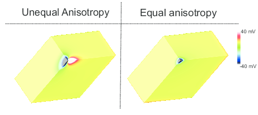
Fig. 69 Induced virtual electrodes in response to a strong hyperpolarizing extracellular stimulus for the equal and unequal anisotropy ratios.

Run anisotropy ratio examples

To compute longitudinal and transverse conductivities for the case of equal anisotropy ratios and $CV_f = 0.6$ and $CV_s = 0.3$ , run

./run.py --ar=1.0

You should get conductivities similar to these:

g_if: 0.152700  g_is: 0.036500  g_ef: 0.548500  g_es: 0.131100

To compute longitudinal and transverse conductivities for the case of unequal anisotropy ratios and $CV_f = 0.6$ and $CV_s = 0.3$ , run

./run.py --ar=3.0

You should get conductivities similar to these:

g_if: 0.152700  g_is: 0.031200  g_ef: 0.548500  g_es: 0.336100

References

[1]	(1, 2, 3, 4) Costa CM, Hoetzl E, Rocha BM, Prassl AJ, Plank G., Automatic Parameterization Strategy for Cardiac Electrophysiology Simulations, Comput Cardiol 40:373-376, 2013. [Pubmed]

[2]	B. J. Caldwell, M. L. Trew, G. B. Sands, D. A. Hooks, I. J. LeGrice, B. H. Smaill, Three distinct directions of intramural activation reveal nonuniform side-to-side electrical coupling of ventricular myocytes., Circ Arrhythm Electrophysiol, vol. 2, no. 4, pp. 433-440, Aug 2009. [Pubmed]