CME - Manual
Modeling Cardiac Function

Model Parameterization and Initialization
While generic models using generic parameter sets and initial values can be valuable and provide generic mechanistic insights, other applications prompt for using specific parameter sets and initial values to facilitate model-based predictions on a case-by-case basis. In such application such as the use of modeling in the clinic as a tool for planning and optimizing therapies, stratification of patients and the prediction of outcomes it is necessary to personalize models, that is, to tune the model behaviour for a specific individual. Within the equations presented, many parameters are required which are based on physiology. However, getting accurate estimates of these is challenging for many reasons as discussed below:
- Anatomical variability: The heart is an organ of high plasticity
which changes its anatomical shape over a lifetime as a function of the imposed workload.
If a heart is overloaded by either volume or pressure to cause stresses or strains within the myocardium
above a critical threshold, remodelling processes are triggered leading to concentric or eccentric shape changes of the ventricles.
Apart from pathological alterations in shape due to congenital malformations or pathological overload conditions,
cardiac anatomy varies significantly not only between species,
but also between individuals of the same species.
Clinical modeling applications attempt to represent an individual’s heart anatomy based on tomographic imaging data
as accurately as possible. For such applications specialized model building workflows have been developed
which seek to build anatomical models of a given patient’s heart as automated as possible
to minimize the need for operator interventions (See
fig-model-building). - Spatial heterogeneity: Cells naturally possess differences with no two cells perfectly equal. Shape and protein expression differ between cells in the same region, due to the slightly different environments seen and the stochastic nature of cellular processes. Across larger spatial scales, clear gradients are observed, as from the apex to the base, from the endocardium to the epicardium, and between the left and right ventricles. Furthermore, protein expression levels also follow a circadian rhythm which can be significant, so sample acquisition time is a factor.
- Incompleteness of data: A complete data set to fully parameterize a cannot be obtained from a single sample. Many samples are require to confidently measure a particular property or quantity, and there are many quantities to measure. Reported values are averages, but given the nonlinear behaviour of biological systems, there is no guarantee that using averaged properties result in typical behaviour.
- Sample preparation: Experiments to determine parameter values require disruption of the natural state of the heart. Even with in tact hearts, function is severely affected. Simply opening the torso affects thoracic pressure with consequences. Excising a heart, i.e. a Langendorff set up, removes the influence of circulating hormones, and neurotransmitters, as well as eliminates central nervous input. Furthermore, performance degrades over time as the blood supply is disrupted leading to reduced energy stores and accumulation of waste products. Tissue preparations go further in removing mechanical load. With single cell preparations, the isolation procedure involves digestion of the interstitial collagen which also changes cell shape. Protein turnover of membrane channels is highly dynamic, over a time scale of minutes, and isolation affects ion channel expression.
- Tissue structure: The rotating transmural predominant fibre orientation makes direct measurements of material quantities impossible since the properties are anisotropic and dictated by cellular direction which change significantly over the distance of microns. A fibre orientation distribution must be assumed. For example, one cannot measure conductivity values by simply measuring the voltage associated with an applied current. Estimates of electrical conductivities are bounded to a maximum of 1 S/m but vary widely.
- Clinical Data: For modelling human hearts, clinical data is constrained since measurements cannot be destructive, are limited in time, and tend to be reflect function at the most macroscopic scale. Cadaver hearts are used but their availability is limited, they are usually diseased since they are unsuitable for transplantation, and the pathologies presenting vary widely leading to weak statistical significance. As a result, and not limited to just human models, missing data is supplanted with data from other species which may differ significantly.
- Spatiotemporal scales: Processes in the cell occur at many different time scales, some of which are too fast to accurately measure. Other events may take place over days. Within a cell, important events may occur in nanodomains which are missed if sampled too coarsely.
- Nonspecific and indirect interactions: Drugs or other manipulations are performed to determine parameter values. However, the action may affect more than what is intended. For example, a drug intended to block a particular channel may also affect other channels. Likewise, given the complex feedback systems in biology, a manipulation to one entity may lead to several downstream effects.
CME Components
The main executable carpentry is built for simulating integrated cardiac function covering both multiscale as well as multiphysics aspects. Since many modeling scenarios do not require to take the entire physics into account any additional physics beyond electrophysiology must be explicitly turned on. That is, electrophysiology is always enabled although a configuration may be chosen where tissue remains electrically quiescent, but a plain mechanics simulation without any electrophysiology components is not supported. Some physics functionality of carpentry is exposed to be used in standalone executables, most notably these are bench for modeling single myocyte dynamics or fluid for modeling blood flow.
Technically, the CME structure comprises the shown components: A) Pre-processing tools B) Simulator core components C) Parameterization and initialization engine E) Post-processing tools
This tutorial introduces to the basics of using the carpentry executable for simulating EP at the tissue and organ scale.
Preprocessing
Segmentation and Classification
Meshing
An important step in any modeling endeavor is the generation of discrete representations of the modeling domain. For simple domains we use mesher. For mesh management meshtool is provided.
Multiphysics Mesh Aspects

Conceptual view of relationship between mesh domains in a multiphysics simulation.
Region definition
Active and passive electro-mechanical tissue properties vary throughout the heart. Even under perfectly healthy conditions, action potential shape and duration are variable within the myocardium or conductivities are different between regions of the heart which is reflected in a heterogeneity in conduction velocities. These gradients are due to differences in the intrinsic makeup of cells, changes In general, the exact variation of these properties throughout the heart cannot be determined, however, basic variations of various properties such as AP shape and duration can be measured and such data can be used to characterize the spatial variation of these properties for different regions. For instance, AP shapes can be characterized for cells taken from epicardial, midmyocardial or endocardial tissue, from basal or apical tissue, or from the left or right ventricle.
In computer models mechanisms must be provided to take these known spatial gradients into account.
The main approach implemented in CARPentry relies upon the explicit definition of regions
to which tissue properties can be assigned.
Regions can be formed by defining a set of finite element entities (elements or nodes)
comprising a region. Every finite element entity carries at least one tag
which can be used for region definitions.
If no explicit regions are defined, entities belong to the default region.
There are two distinct approaches to region definition
referred to as Mesh-based tagging and Dynamic tagging.
Mesh-based tagging
Properties are assigned to regions as defined by a set of tags. The properties are assigned homogeneously to the entire region.
Assignment of region tags in a rabbit biventricular slice model.
Dynamic tagging
Dynamic tagging can be used for defining regions on the fly by intersecting geometric primitives
such as spheres, cylinders or blocks with a given mesh.
Users may relabel elements based on specifying a volume and retagging all elements
within the volume, or specifying a list of elements.
The number of user regions to be retagged is controlled by numtagreg and
each region is part of the array tagreg[Int].
With intersecting volumes, the highest region tag takes effect.
For each user-defined tag region, the following fields are defined.
| Field | Type | Description |
|---|---|---|
| tag | int | relabelled tag value |
| name | string | label |
| type | int | volume to define (1=sphere,2=block,3=element list) |
| elemfile | string | file with list of elements to retag |
| p0 | float[3] | center of sphere or LL corner of bounding box |
| p1 | float[3] | UR corner of BB |
| radius | float | radius of sphere |
The use of this dynamic tagging feature is elucidated in the Region tagging tutorial.
Workflows for building anatomically accurate models of the heart typically consist of the following stages: A) Tomographic image stacks based on MRI or CT are acquired to capture anatomy in a given state. Typically, a 3D whole-heart (3DWH) snapshot is taken during diastasis or close to an end-diastolic configuration. Depending on the assumed pathology, often additional scan are available to delineate infarcted tissue (late gadolinium enhancement (LGE) MRI) or fibrosis (T1 mapping). B) 3D image stacks are segmented to delineate the heart from the torso background. C) A more detailed voxel classification is performed to label the various anatomical regions of the heart. Labels are also of pivotal importance for defining the in-silico setup at later processing steps. D) Clinical imaging data tend to be of lower anisotropic resolution and as such are not directly suitable for anatomical mesh generation. Variational smoothing methods are often employed to reduce the jaggedness of the implicit surfaces in the raw segmented image data. E) The smoothed discrete surface representation of the heart is re-rasterized at a high isotropic resolution that is suitable as input for voxel-based mesh generation software. F) 3D finite element meshes are generated that also preserves labeling information added at stage C). G) Tissue properties such as the orientation of local fiber architecture is added, either by rule-or atlas-based methods [1] (Bayer et al), or by mapping of additional information contained in complementary image stacks such as e.g. diffusion-tensor MRI scans. H) Additional features such as topological representations of the His-Purkinje system are mapped onto the 3D FE mesh.
Using CARPentry
In this section the basic usage of the main executable carpentry is explained. More detailed background referring to the individual physics electrophysiology, elasticity and hemodynamics are given below in the respective sections.
Getting Help
As in any real in vivo or ex vivo experiment there is a large number of parameters that have to be set and tracked. In in silico experiments tend to be even higher since not only the measurement setup must be configured, but also the organ itself. The general purpose design of carpentry renders feasible the configuration of a wide range of experimental conditions. Consequently, the number of supported parameters is large, depending on the specific flavor on the order of a few hundreds of parameters that can be used for experimental descriptions. With such a larger number of parameters it is therefore key to be able to retrieve easily more detailed explanations of meaning and intended use of all parameters.
A list of all available command line parameters is obtained by
carpentry +Help

carpentry [+Default | +F file | +Help topic | +Doc] [+Save file]
Default allocation: Global

Parameters:
         -iout_idx_file RFile
         -eout_idx_file RFile
         -output_level Int
         -num_emission_dbc Int
         -num_illum_dbc Int
         -CV_coupling Short
         -num_cavities Int
         -num_mechanic_nbc Int
         -num_mechanic_dbc Int
         -mesh_statistics Flag
         -save_permute Flag
         -save_mapping Flag
         -mapping_mode Short
         ...
         -rt_lib String
         '-external_imp[Int]' String
         -external_imp '{ num_external_imp x String }'
         -num_external_imp Int
and help for a specific feature is queried by
carpentry +Help stimulus[0].strength

stimulus[0].strength:
        stimulus strength

        type:   Float
        default:(Float)(0.)
        units:  uA/cm^2(2D current), uA/cm^3(3D current), or mV
        Depends on: {
                stimulus[PrMelem1]
        }
More verbose explanation of command line parameters is obtained by using the +Doc parameter
which prints the same output as +Help, but provides in addition more details on each individual parameter:
carpentry +Doc

iout_idx_file:
        path to file containing intracellular indices to output

        type:   RFile
        default:(RFile)("")


eout_idx_file:
        path to file containing extracellular indices to output

        type:   RFile
        default:(RFile)("")


output_level:
        Level of terminal output; 0 is minimal output

        type:   Int
        default:(Int)(1)
        min:    (Int)(0)
        max:    (Int)(10)


num_emission_dbc:
        Number of optical Dirichlet boundary conditions

        type:   Int
        default:(Int)(0)
        min:    (Int)(0)
        max:    (Int)(2)
        Changes the allocation of: {
                emission_dbc
                emission_dbc[PrMelem1].bctype
                emission_dbc[PrMelem1].geometry
                emission_dbc[PrMelem1].ctr_def
                emission_dbc[PrMelem1].zd
                emission_dbc[PrMelem1].yd
                emission_dbc[PrMelem1].xd
                emission_dbc[PrMelem1].z0
                emission_dbc[PrMelem1].y0
                emission_dbc[PrMelem1].x0
                emission_dbc[PrMelem1].strength
                emission_dbc[PrMelem1].dump_nodes
                emission_dbc[PrMelem1].vtx_file
                emission_dbc[PrMelem1].name
        }
        Influences the value of: {
                emission_dbc
        }
Details on the executable and the main features it was compiled with are queried by
carpentry -revision

svn revision:             2974
svn path:                 https://carpentry.medunigraz.at/carp-dcse-pt/branches/mechanics/CARP
dependency svn revisions: PT_C=338,elasticity=336,eikonal=111
Basic experiment definition
Various types of experiments are supported by carpentry. A list of experimental modes is obtained by
carpentry +Help experiment
yielding the following list:
| Value | Description |
|---|---|
| 0 | NORMAL RUN (default) |
| 1 | Output FEM matrices only |
| 2 | Laplace solve |
| 3 | Build model only |
| 4 | Post-processing only |
| 5 | Unloading (compute stress-free reference configation) |
| 6 | Eikonal solve (compute activation sequence only) |
| 7 | Apply deformation |
| 8 | memory test (obsolete?) |
A representation of the tissue or organ to be modelled must be provided in the form of a finite element mesh that adheres to the primitive carpentry mesh format. The duration of activity to be simulated is chosen by -tend which is specified in milli-seconds. Specifying these minimum number of parameters already suffices to launch a basic simulation
carpentry -meshname slab -tend 100
Due to the lack of any electrical stimulus this experiment only models electrophysiology in quiescent tissue and, in most cases, such an experiment will be of very limited interest. However, carpentry is designed based on the notion that any user should be able to run a simple simulation by providing a minimum of parameters. This was achieved by using the input parser prm through which reasonable default settings for all parameters must be provided and inter-dependency of parameters and potential inconsistencies are caught immediately when launching a simulation. This concept makes it straight forward to define an initial experiment easily and implement then step-by-step incremental refinements until the desired experimental conditions are all matched.
Picking a model and discretization scheme
carpentry +Help bidomain
# explain operator splitting, mass lumping,
The time stepping for the parabolic PDE is chosen with -parab_solv. There are three options available.
Picking a solver
The carpentry solver infrastructure relies largely on preconditioners and solvers made available through PETSc. However, in many cases there are alternative solvers available implemented in the parallel toolbox (PT). Whenever PT alternatives are available we typically prefer PT for several reasons:
- Algorithms underlying PT are developed by our collaborators, thus it is easier to ask for specific modifications/improvements, if needed
- PT is optimized for strong scalability, in many cases we achieve better performance with lightweight PT solvers then with PETSc solvers. In general, PT needs more iteration, but each iteration is cheaper.
- PT is fully GPU enabled.
Switching between PETSc/PT solvers is achieved with
PETSc solvers can be configured by feeding in option files at the command line. These option files are passed in using the following command line arguments
| ellip_options_file parab_options_file purk_options_file |
There are three options available.
After selecting a solver, for each physical problem convergence criteria are chosen and the maximum number of allowed iterations can be defined.
Configuring IO
Cardiac Electrophysiology Modeling
Single Cell Scale - Ionic Models
For electrophysiological simulation, the basic unit of the model is the cellular activity. Cellular models of cardiac electrical activity were first constructed over 50 years ago, and today, these models have been refined and are routinely put into organ scale simulations. The modelling components are described below.
Ionic models refer to the electrical representation of the cell based on the movement of ions across the cell membrane, resulting in a change in the voltage across the membrane. Schematically, a capacitor is placed in parallel with a number of ionic transport mechanisms. In general, an ionic model is of the form
()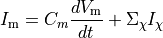
where  is the voltage across the cell membrane,
 is the net current across the membrane,
 is the membrane capacitance,
and
is the membrane capacitance,
and  is a particular transport mechanism, either a channel, pump or exchanger.
Additional equations may track ionic concentrations and the processes which affect them,
like calcium-induced release from the sarcoplasmic reticulum.
By convention, outward current, i.e., positive ions leaving the cell, is defined as being positive, while inward currents are negative.
is a particular transport mechanism, either a channel, pump or exchanger.
Additional equations may track ionic concentrations and the processes which affect them,
like calcium-induced release from the sarcoplasmic reticulum.
By convention, outward current, i.e., positive ions leaving the cell, is defined as being positive, while inward currents are negative.
Channels are represented as resistors in series with a battery. The battery represents the Nernst Potential resulting from the electrical field developed by the ion concentration difference across the membrane. It is given by
()¶![\begin{equation}
E_S = \frac{RT}{zF}\ln\frac{[S]_i}{[S]_e} \nonumber
\end{equation}](_images/math/4dafc5d04367cbc739a36281b672218e1392c089.png)
where  is the gas constant,
 is the temperature,
 is Faraday’s constant and
  is the valence of the ion species
  .
Channels are dynamical systems which open and close in response to various conditions
like transmembrane voltage, stretch, ligands, and other factors.
The opening and closing rates of the channels vary by several orders of magnitudes, and are generally, nonlinear in nature.
Thus, the equivalent electrical resistance of a channel is a time dependent quantity.
.
Channels are dynamical systems which open and close in response to various conditions
like transmembrane voltage, stretch, ligands, and other factors.
The opening and closing rates of the channels vary by several orders of magnitudes, and are generally, nonlinear in nature.
Thus, the equivalent electrical resistance of a channel is a time dependent quantity.
The first representation of a cardiac cell was that produced by D. Noble of a Purkinje cell, based on modification of the Hodgkin-Huxley nerve action potential. Since then, hundreds of models have been developed for many reasons. Ionic models need to be developed to match experimental procedures if the models are to be predictive and offer insight into mechanistic workings. In mammals, action potential durations range from tens of milliseconds for mice to several hundreds of milliseconds for large animals. Atrial myocyte protein expression is quite different from that of ventricular myocytes, resulting in different action potential durations and shapes. Even nearby cells exhibit action potential differences due to slightly different levels of channel protein expression. The complexity of ionic models has been steadily growing as more knowledge is gained through better experimental techniques, equipment and specific blockers of transport mechanisms. As more mechanisms are identified as affecting electrophysiology, either directly or indirectly, they are incorporated into ionic models. Selection of the model to use is not always obvious as different models may be available for the same species and heart location, which may yield quite different behaviour. Regardless, identifying the strengths and weaknesses of an ionic model for a particular application is important.
Ionic models may be biophysically detailed or phenomenological. Biophysically detailed models attempt to discretely depict important currents and processes within the cell. Early models had approximately ten equations depicting only sodium and potassium channels, while present models have hundreds of equations taking into account not only membrane ion transporters, but intracellular calcium handling, mitochondrial function, and biochemical signalling pathways. Conversely, phenomenological ionic models use a set of currents which faithfully reproduce whole cell behaviour in terms of action potential shape and duration, and restitution properties. The currents in the phenomenological model are not physiological but can be considered as amalgamations of known currents. While these models are computationally much simpler and easier to tune, they lose the direct correspondence with the biophysics which makes implementing drug effects or cellular pathologies challenging. Finally, cellular automata models have also been used, and can be considered as a type of phenomenological model. These models do not use differential equations but have a set of rules which dictate transitions between discrete states of the model. As such, these models are computationally light, and can be as detailed as required. However, behaviour may not be as rich as differential equations. The choice of model, biophysical or phenomenological, depends on the nature of the problem being considered, and the availability of computational resources for the problem size.
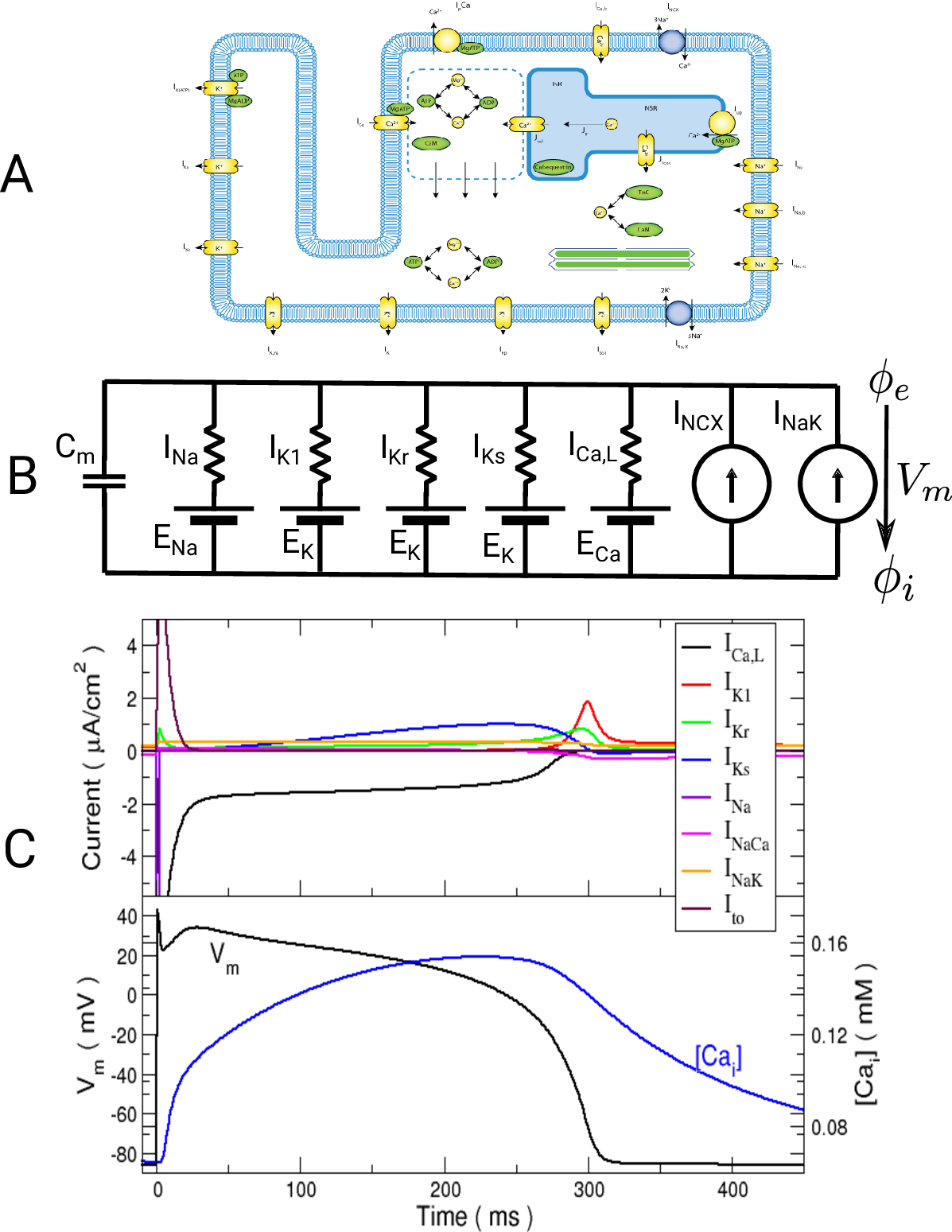
Ionic models A: Myocyte schematic showing the membrane (blue) which contains channels (yellow cylinders),
pumps (yellow circles) and exchangers (blue circles).
The sarcoplasmic reticulum is divided into the junctional (JSR) and network (NSR) regions
and channels and pumps control ion movement into and out of it.
Figure taken from
Michailova et al.
B: Electrical representation of a cell showing a limited number of currents:
fast sodium ( ),
inward rectifier (
),
inward rectifier ( ),
fast and slow repolarizing currents (
),
fast and slow repolarizing currents ( and
and  )
L-type calcium (
)
L-type calcium ( },
the sodium-potassium pump (
},
the sodium-potassium pump ( ) and the sodium-calcium exchanger (
 ).
Nernst potentials for the ionic species are indicated (
).
Nernst potentials for the ionic species are indicated ( ) as is the membrane capacitance ().
C: Effect of applying a suprathreshold current at time 0 to the ten Tuscher ionic model of the human ventricular myocyte.
Top: Major ionic currents. Note that the following currents are clipped:
) as is the membrane capacitance ().
C: Effect of applying a suprathreshold current at time 0 to the ten Tuscher ionic model of the human ventricular myocyte.
Top: Major ionic currents. Note that the following currents are clipped:
 (-46.4),
  (15.3), and (-9.6).
Bottom: the resulting action potential () and myoplasmic calcium transient (
(15.3), and (-9.6).
Bottom: the resulting action potential () and myoplasmic calcium transient (![[Ca_{\rm i}]](_images/math/de0023b1b167317826d96b7479be82cbf11eeb2b.png) ). }
). }
When considering the mathematical description of ionic channels, there are two main approaches which are detailed below.
Hodgkin-Huxley Dynamics
The Hodgkin-Huxley approach is named after the Nobel laureates
who were the first to develop a mathematical model of the neural action potential.
Single channel activity recordings show that channels have a small set of discrete conductance states, with
the channel stochastically transitioning between closed states and open states.
Short time analysis of a single channel is very difficult to interpret
but ensemble averaging clearly reveals smooth kinetics in changes of channel conductance.
In the Hodgkin-Huxley formulation, channel conductance
is assumed to be controlled by gates which take on values between 0 and unity, representing the portion of the cells in one state.
Since cells have hundreds of ion channels if not more, this approximation holds well.
Current flow produced by ion species  passing through a channel is then described by
()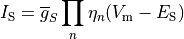
where  is the maximum conductance of the channel and
  is a gating variable.
Often the gating variable is assumed to follow first order dynamics so
is a gating variable.
Often the gating variable is assumed to follow first order dynamics so
()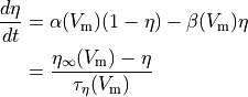
where  and
and  are rates
which can be cast into an equivalent form of a steady state value (
are rates
which can be cast into an equivalent form of a steady state value ( )
and a rate of change (
)
and a rate of change ( ).
The advantage of this latter formulation is that mathematically,
the update of the gating variables can be performed by a numercial integration method,
the Rush-Larsen technique, which is guaranteed to unconditionally keep the gating variable bounded
within the range [0,1] while allowing a large time step.
).
The advantage of this latter formulation is that mathematically,
the update of the gating variables can be performed by a numercial integration method,
the Rush-Larsen technique, which is guaranteed to unconditionally keep the gating variable bounded
within the range [0,1] while allowing a large time step.
Markov Models
Markov models describe the channel as a set off states, such as the conductance states seen in single channel recordings, as well as the non conducting states through which a channel must pass to reach them. Transitions between states are described by rate constants which can be functions of concentrations or voltages, or fixed. These is a variables for each state which represent the portion of channels in a cell which are in that state. As such, the sum of state variables is unity. A Hodgkin-Huxley made can be converted to a Markov model by considering a gating variable as a two state model. However, the advantage of the Markov representation is its ability to model drug interaction. Essentially, drug binding doubles the number of possible states in an ionic model, augmenting the original states with drug-bound versions. One may easily limit drug binding to a particular subset of channel states, and more finely control channel kinetics.
Single Cell modeling tool bench
The single cell experimentation tool bench is quite versatile and can be used
to replicate a wider range of single cell experimental protocols.
A tutorial on how to use bench is given here.
The following sections demonstrate how one explores all available
bench functions and explains the command line arguments available.
Getting Help
The --help, --detailed-help or --full-help arguments provide a list of all available arguments
with increasing levels of detail.
bench --help

LIMPET 1.1

Use the IMP library for single cell experiments. All times in ms; all voltages
in mV;  currents in uA/cm^2

Usage: LIMPET [-h|--help] [--detailed-help] [--full-help] [-V|--version]
         [-cFLOAT|--stim-curr=FLOAT] [--stim-volt=FLOAT] [--stim-file=STRING]
         [-aDOUBLE|--duration=DOUBLE] [-DDOUBLE|--dt=DOUBLE] [-nINT|--num=INT]
         [--ext-vm-update] [--rseed=INT] [-TDOUBLE|--stim-dur=DOUBLE]
         [-A|--stim-assign] [--stim-species=STRING] [--stim-ratios=STRING]
         [--resistance=DOUBLE] [-ISTRING|--imp=STRING]
         [-pSTRING|--imp-par=STRING] [-PSTRING|--plug-in=STRING]
         [-mSTRING|--plug-par=STRING] [--load-module=STRING]
         [-lDOUBLE|--clamp=DOUBLE] [-LDOUBLE|--clamp-dur=DOUBLE]
         [--clamp-start=DOUBLE] [--clamp-SVs=STRING] [--SV-clamp-files=STRING]
         [--SV-I-trigger] [--AP-clamp-file=STRING] [-NDOUBLE|--strain=DOUBLE]
         [-tDOUBLE|--strain-time=DOUBLE] [-yFLOAT|--strain-dur=FLOAT]
         [--strain-rate=DOUBLE] [-oDOUBLE|--dt-out=DOUBLE]
         [-OSTRING|--fout=STRING] [--no-trace] [--trace-no=INT] [-B|--bin]
         [-uSTRING|--imp-sv-dump=STRING] [-gSTRING|--plug-sv-dump=STRING]
         [-d|--dump-lut] [--APstatistics] [-v|--validate]
         [-sDOUBLE|--save-time=DOUBLE] [-fSTRING|--save-file=STRING]
         [-rSTRING|--restore=STRING] [-FSTRING|--save-ini-file=STRING]
         [-SDOUBLE|--save-ini-time=DOUBLE] [-RSTRING|--read-ini-file=STRING]
         [--SV-init=STRING]
  or : LIMPET [--list-imps] [--plugin-outputs] [--imp-info]
  or : LIMPET [--stim-times=STRING]
  or : LIMPET [--numstim=INT] [-iDOUBLE|--stim-start=DOUBLE]
         [-bDOUBLE|--bcl=DOUBLE]
  or : LIMPET --restitute=STRING [--res-file=STRING] [--res-trace]
  or : LIMPET --clamp-ini=DOUBLE --clamp-file=STRING

  -h, --help                   Print help and exit
      --detailed-help          Print help, including all details and hidden
                                 options, and exit
      --full-help              Print help, including hidden options, and exit
  -V, --version                Print version and exit

 Mode: regstim
  regular periodic stimuli
      --numstim=INT            number of stimuli  (default=`1')
  -i, --stim-start=DOUBLE      start stimulation  (default=`1.')
  -b, --bcl=DOUBLE             basic cycle length  (default=`1000.0')

 Mode: neqstim
  irregularly timed stimuli
      --stim-times=STRING      comma separated list of stim times  (default=`')

 Mode: restitute
  restitution curves
      --restitute=STRING       restitution experiment  (possible
                                 values="S1S2", "dyn", "S1S2f")
      --res-file=STRING        definition file for restitution parameters
                                 (default=`')
      --res-trace              output ionic model trace  (default=off)

 Mode: info
  output IMP information
      --list-imps              list all available IMPs  (default=off)
      --plugin-outputs         list the outputs of available plugins
                                 (default=off)
      --imp-info               print tunable parameters and state variables for
                                 particular IMPs  (default=off)

 Mode: vclamp
  Constant Voltage clamp
      --clamp-ini=DOUBLE       outside of clamp pulse, clamp Vm to this value
                                 (default=`-80.0')
      --clamp-file=STRING      clamp voltage to a signal read from a file
                                 (default=`')

 Group: stimtype
  stimulus type
  -c, --stim-curr=FLOAT        stimulation current  (default=`60.0')
      --stim-volt=FLOAT        stimulation voltage
      --stim-file=STRING       use signal from a file for current stim

Simulation control:
  -a, --duration=DOUBLE        duration of simulation  (default=`1000.')
  -D, --dt=DOUBLE              time step  (default=`.01')
  -n, --num=INT                number of cells  (default=`1')
      --ext-vm-update          update Vm externally  (default=off)
      --rseed=INT              random number seed  (default=`1')

Stimuli:
  -T, --stim-dur=DOUBLE        duration of stimulus pulse  (default=`1.')
  -A, --stim-assign            stimulus current assignment  (default=off)
      --stim-species=STRING    concentrations that should be affected by
                                 stimuli, e.g. 'K_i:Cl_i'  (default=`K_i')
      --stim-ratios=STRING     proportions of stimlus current carried by each
                                 species, e.g. '0.7:0.3'  (default=`1.0')
      --resistance=DOUBLE      coupling resistance [kOhm]  (default=`100.0')

Ionic Models:
  -I, --imp=STRING             IMP to use  (default=`MBRDR')
  -p, --imp-par=STRING         params to modify IMP  (default=`')
  -P, --plug-in=STRING         plugins to use, separate with ':'  (default=`')
  -m, --plug-par=STRING        params to modify plug-ins, separate params with
                                 ',' and plugin params with ':'  (default=`')
      --load-module=STRING     load a module for use with bench (implies --imp)
                                 (default=`')

Voltage clamp pulse:
  -l, --clamp=DOUBLE           clamp Vm to this value  (default=`0.0')
  -L, --clamp-dur=DOUBLE       duration of Vm clamp pulse  (default=`0.0')
      --clamp-start=DOUBLE     start time of Vm clamp pulse  (default=`10.0')

Clamps:
      --clamp-SVs=STRING       colon separated list of state variable to clamp
                                 (default=`')
      --SV-clamp-files=STRING  : separated list of files from which to read
                                 state variables  (default=`')
      --SV-I-trigger           apply SV clamps at each current stim
                                 (default=on)
      --AP-clamp-file=STRING   action potential trace applied at each stimulus
                                 (default=`')

Strain:
  -N, --strain=DOUBLE          amount of strain to apply  (default=`0')
  -t, --strain-time=DOUBLE     time to strain  (default=`200')
  -y, --strain-dur=FLOAT       duration of strain (default=tonic) [ms]
      --strain-rate=DOUBLE     time to apply/remove strain  (default=`2')

Output:
  -o, --dt-out=DOUBLE          temporal output granularity  (default=`1.0')
  -O, --fout[=STRING]          output to files  (default=`BENCH_REG')
      --no-trace               do not output trace  (default=off)
      --trace-no=INT           number for trace file name  (default=`0')
  -B, --bin                    write binary files  (default=off)
  -u, --imp-sv-dump=STRING     sv dump list  (default=`')
  -g, --plug-sv-dump=STRING    : separated sv dump list for plug-ins, lists
                                 separated by semicolon  (default=`')
  -d, --dump-lut               dump lookup tables  (default=off)
      --APstatistics           compute AP statistics  (default=off)
  -v, --validate               output all SVs  (default=off)

State saving/restoring:
  -s, --save-time=DOUBLE       time at which to save state  (default=`0')
  -f, --save-file=STRING       file in which to save state  (default=`a.sv')
  -r, --restore=STRING         restore saved state file  (default=`a.sv')
  -F, --save-ini-file=STRING   text file in which to save state of a single
                                 cell  (default=`singlecell.sv')
  -S, --save-ini-time=DOUBLE   time at which to save single cell state
                                 (default=`0.0')
  -R, --read-ini-file=STRING   text file from which to read state of a single
                                 cell  (default=`singlecell.sv')
      --SV-init=STRING         colon separated list of comma separated
                             SV=initial_values
Available models
The --list-imps argument outputs a list of all available ionic models and plugins.
bench --list-imps

Ionic models:
    AlievPanfilov
    ARPF
    Steward
    converted_COURTEMANCHE
    converted_DiFranNoble
    converted_LRDII_F
    converted_MBRDR
    converted_NYGREN
    converted_RNC
    converted_TT2
    converted_UCLA_RAB
    UCLA_RAB_SCR
    COURTEMANCHE
    DiFranNoble
    ECME
    FHN_RMcC
    FOX
    GPB
    GPVatria
    GPB_Land
    GW_CAN
    hAMr
    HH
    IION_SRC
    INADA_AVN
    Iribe
    JBTT2
    Kurata
    LMCG
    LR1
    LRDII
    LRDII_F
    MacCannell_Fb
    MitchellSchaeffer
    mMS
    MBRDR
    MurineMouse
    NYGREN
    ORd
    Pandit
    PASSIVE
    PUG
    Rat_neon
    RNC
    SC
    TT2
    TT
    TTRED
    UCLA_RAB
    WANG_NNR
    SHANNON
    GTT2_fast
    GTT2_fast_PURK
    JB_COURTEMANCHE
Plug-ins:
    converted_EP
    converted_EP_RS
    converted_IA
    EP
    EP_RS
    ExcConNHS
    I_ACh
    IA
    IFun
    I_KATP
    INa_Bond_Markov
    I_NaH
    Muscon
    NPStress
    FxStress
    TanhStress
    Rice
    LandStress
    NHSstress
    Lumens
    SAC_KS
    YHuSAC
Show model state variables and exposed parameters
The --imp-info argument lists all state variables of a model
and all exposed parameters which can be modified.
For instance, to interrogate this for the tenTusscher 2 model run:
bench --imp TT2 --imp-info

TT2:
                                 big_cnt        0
                                   fmode        0
                                      Ko        5.4
                                     Cao        2
                                     Nao        140
                                      Vc        0.016404
                                     Vsr        0.001094
                                    Bufc        0.2
                                   Kbufc        0.001
                                   Bufsr        10
                                  Kbufsr        0.3
                                  Vmaxup        0.006375
                                     Kup        0.00025
                                       R        8314.47
                                       F        96485.3
                                       T        310
                                   RTONF        26.7138
                             CAPACITANCE        0.185
                                     Gkr        0.153
                                    pKNa        0.03
                                     Gks        0.392
                                     GK1        5.405
                                     Gto        0.294
                                     GNa        14.838
                                    GbNa        0.00029
                                     KmK        1
                                    KmNa        40
                                    knak        2.724
                                    GCaL        3.98e-05
                                    GbCa        0.000592
                                   knaca        1000
                                   KmNai        87.5
                                    KmCa        1.38
                                    ksat        0.1
                                       n        0.35
                                    GpCa        0.1238
                                    KpCa        0.0005
                                     GpK        0.0146
                               scl_tau_f        1
                                   flags        ENDO|EPI|MCELL
        State variables:
                                Ca_i
                                CaSR
                                CaSS
                                  R_
                                   O
                                Na_i
                                 K_i
                                   M
                                   H
                                   J
                                 Xr1
                                 Xr2
                                  Xs
                                   R
                                   S
                                   D
                                   F
                                  F2
                               FCaSS
The --plugin-outputs argument provides the same information as --imp-info,
but lists in addition all the outputs of plugins, that is,
global quantities modified by a given plugins.
Plug-ins:
        converted_EP     Iion
        converted_EP_RS  Iion
        converted_IA     Iion
        EP               Iion
        EP_RS            Iion
        ExcConNHS        Tension
        I_ACh            Iion
        IA               Iion
        IFun             Iion
        I_KATP           K_e Iion
        INa_Bond_Markov  Iion
        I_NaH            Na_e
        Muscon           Tension
        NPStress         Tension
        FxStress         Tension
        TanhStress       Tension
        Rice             Tension
        LandStress       Tension
        NHSstress        Tension
        Lumens           delLambda Tension
        SAC_KS           Iion
        YHuSAC           Iion
Define a stimulus
The arguments --stim-curr and --stim-volt select the magnitude of a current or voltage stimulus pulse
in  and
and  , respectively.
The duration of a stimulus is set through the
, respectively.
The duration of a stimulus is set through the stim-dur argument.
Alternatively, a trace file can be provided through --stim-file to impose a stimulus of arbitrary shape.
To initiate an action potential in the TT2 model by applying a current stimulus of  and 2 ms duration run
bench --stim-curr 60 --stim-dur 2
or, to stimulate with an arbitrary stimulus current profile run
bench --stim-file mypulse.trc
where the stimulus definition file mypulse.trc must comply with the following format:
#samples
t0  y0
t1  y1
t2  y2
...
tN  yN
Define a stimulus protocol
Two types of protocols are supported, a train of regular periodic stimuli or a train of irregularly time stimuli.
In the regular case the total number of stimuli to be delivered is prescribed by --numstim
and the interval between stimuli by the basic cycle length argument --bcl.
The stimulus protocol is initiated at a given time prescribed by --stim-start.
bench --imp TT2 --numstim 50 --stim-start 10. --bcl 350
An irregular stimulus sequence is specified through the --stim-times argument.
bench --imp TT2 --stim-times 10,360,700,920
The response to this stimulus definition is illustrated here.
When using the --stim-times options the number of stimuli depends solely on the times provided,
using the --num-stim causes a conflict.

Irregular basic cycle length due to stimulation using --stim-times.
Read the default command line output
Depending on the ionic model and the plugins used global variables which may diffuse at the tissue level are written to the console. The output will look similar to
bench --imp TT2

Outputting the following quantities at each time:
   Time              Vm            Iion

  0.000 -8.62000000e+01 +0.00000000e+00
  1.000 -8.61618521e+01 -3.46181728e-02
  2.000 +4.10176938e+01 -6.35646133e+01
  3.000 +3.51969845e+01 +1.22923870e+01
  4.000 +2.62015535e+01 +5.84205961e+00
  5.000 +2.29077661e+01 +1.52032351e+00
...
To quickly visualize AP shape or ionic current redirect the output to a file and visualize with your preferred tool.
Basic stimulation control
The overall duration of simulation is set by --duration in [ms] and the integration time step is chosen by --dt in [ms].
The time stepping method cannot be chosen at the command line as ODE integration in LIMPET is hardcoded,
but the source code for any ionic model can be regenerated with a different integration scheme
(see limpet_fe.py for details). To simulate 10 action potentials at a basic cycle length of 500 ms
the overall duration of the simulation should be picked as  .
.
bench --duration 5000 --bcl 500 --num-stim 10 --stim-start 0
Simple AP visualization
To quickly visualize the shape of an action potential or the ionic current redirect the output to a file
bench --duration 400 --dt-out 0.1 --fout=AP
Time  , transmembrane voltage
  and ionic current,
  are written to the file
 AP.txt. Use your favourite plotting tool such as, for instance, gnuplot.
gnuplot

# plot Vm
plot 'AP.txt' using 1:2 with lines

# plot Iion
plot 'AP.txt' using 1:3 with lines
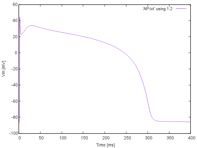
Simple AP visualization with gnuplot
Performance benchmarking
For the sake of performance benchmarking the number of cell solved can be increased using --num.
Performance metrics of the ODE solver are reported in any simulation run at the end of the output.
To run a short benchmark simulating 10 ms of activity in 10000 cells use:
mpiexec -n 16 bench --num 100000 --duration 10
This outputs a basic performance statistics as shown below:
setup time          0.001208 s
initialization time 0.036891 s
main loop time      2.801997 s
total ode time      2.788086 s

mn/avg/mx loop time 2.064943 2.799198 5.839109 ms
mn/avg/mx ODE time  2.063036 2.785301 5.825996 ms
real time factor    0.003587
Model modification
Model behavior can be modified by providing parameter modification string through --imp-par.
Modifications strings are of the following form:
param[+|-|/|*|=][+|-]###[.[###][e|E[-|+]###][\%]
where param is the name of the parameter one wants to modify
such as, for instance, the peak conductivity of the sodium channel, GNa.
Not all parameters of ionic models are exposed for modification,
but a list of those which are can be retrieved for each model using imp-info.
As an example, let’s assume we are interested in specializing a generic human ventricular myocyte
based on the ten Tusscher-Panfilov model to match the cellular dynamics of myocytes
as they are found in the halo around an infarct, i.e.in the peri-infarct zone (PZ).
In the PZ various current are downregulated.
Patch-clamp studies of cells harvested from the peri-infract zone have reported
a 62% reduction in peak sodium current, 69% reduction in L-type calcium current
and a reduction of 70% and 80% in potassium currents  and
and  , respectively.
In the model these modifications are implemented by altering the peak conductivities of the respective currents as follows:
, respectively.
In the model these modifications are implemented by altering the peak conductivities of the respective currents as follows:
# all modification strings yield the same results
bench --imp TT2 --imp-par="GNa-62%,GCaL-69%,Gkr-70%,GK1-80%" --numstim 10 --bcl 500 --duration 5000

# or
bench --imp TT2 --imp-par="GNa*0.38,GCaL*0.31,Gkr*0.3,GK1*0.2" --numstim 10 --bcl 500 --duration 5000
To make sure that the provided parameter modifications are used as expected look at the log messages printed to the console. You should see messages confirming the use of the specified parameter modifications:
Ionic model: TT2
        GNa                  modifier: -62%            value: 5.63844
        GCaL                 modifier: -69%            value: 1.2338e-05
        Gkr                  modifier: -70%            value: 0.0459
        GK1                  modifier: -80%            value: 1.081
To observe the effect of the modification relative to the baseline model simulate a train of action potentials with both baseline and modified model. Run
# run baseline model
bench --imp TT2 --numstim 10 --bcl 500 --duration 5000 --fout=TT2_baseline

# run modified PZ model
bench --imp TT2 --imp-par="GNa-62%,GCaL-69%,Gkr-70%,GK1-80%" --numstim 10 --bcl 500 --duration 5000 --fout=TT2_PZ
fig-TT2-PZone illustrates the effect of the parameter modifications upon AP features.
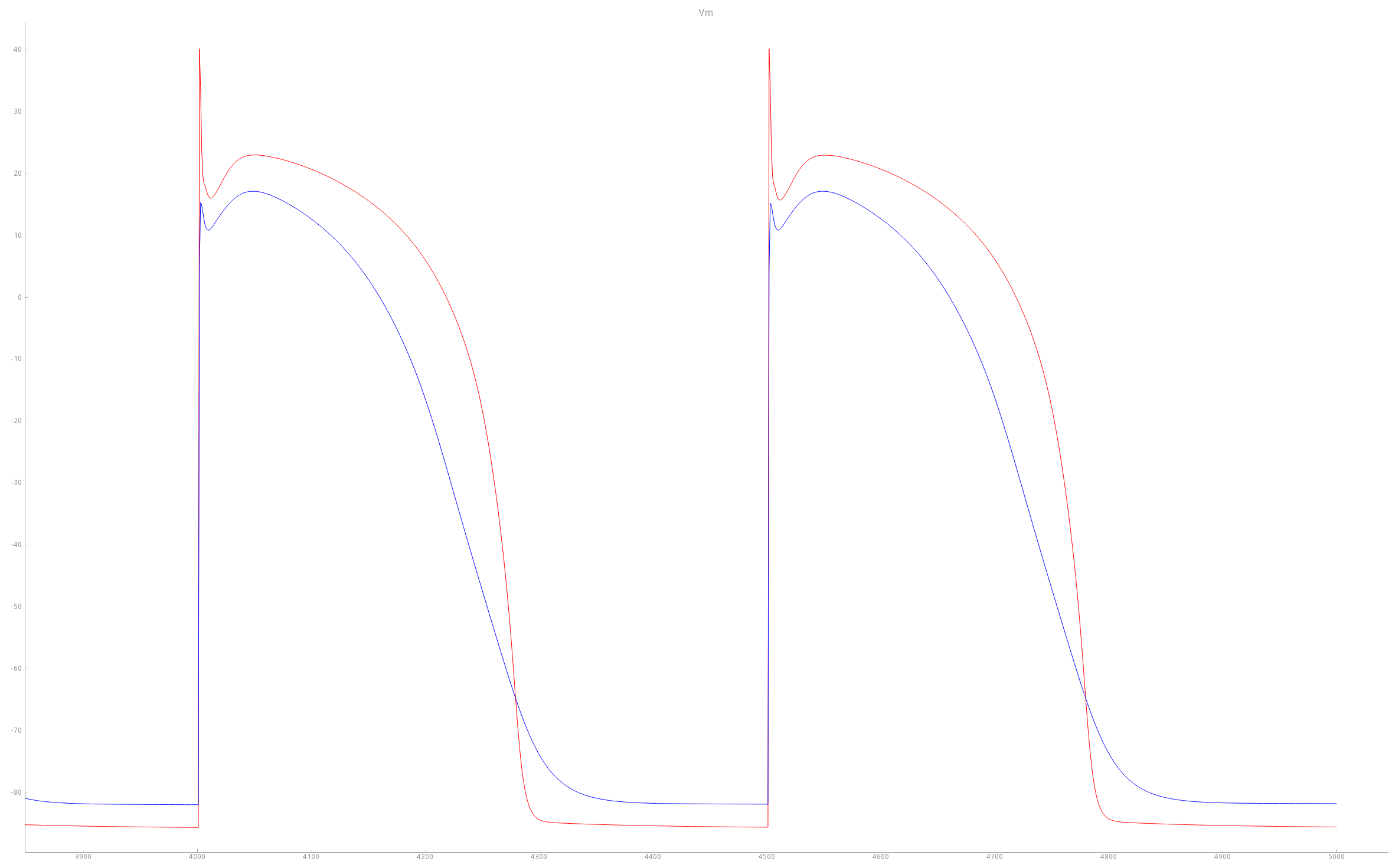
Comparison of TT2 APs with baseline (red trace) and modified PZ (blue trace) settings. As a result of the modifications, the PZ APs feature a longer duration, decreased upstroke velocity and decreased peak amplitude compared to baseline APs.
Model augmentation
Published models of cellular dynamics are not complete and comprehensive representations
of the electrophysiological behavior of a myocyte.
Rather, the represent a subset of features which were deemed relevant for a given purpose.
This is true for any published model, none of them is able to represent myocyte behavior
under an arbitrary range of experimental circumstances.
For the sake of verification it is crucial to be able to run models
under the exact same conditions under which published results were obtained.
However, after verification it is often necessary to augment a model with additional features
which remained unaccounted for in the original publication.
The --plug-in mechanism is designed for such applications
where additional currents or physical effects such as the generation of active tension are considered
without recompiling or directly modifying the model as published.
The underlying concept is illustrated in fig-augment.
Typical augmentation is used for incorporating additional currents which play a role
when driving the transmembrane potential beyond the physiological range
during the application of a strong depolarizing/hyperpolarizing stimuli
such as an electroporation current, EP,
an electroporation current with pore resealing, EP_RS,
or a hypothetical time-independent outward rectifying potassium current IA,
or to account for the effect of adrenergic stimulation by incorporating
an acetylcholine-dependent potassium current I_ACh

Design concept underlying the implmented augmentation mechanism in LIMPET.
For instance, to augment a model of cellular dynamics to be used for studying the effect of defibrillation shocks,
one would activate the plugins EP_RS and IA.
This is achieved as follows:
bench --imp TT2 --plug-in "EP_RS:IA"
A frequent use of plugins is the augmentation with active stress models.
For instance, to specialize a human ventricular myocyte model for use in a ventricular electro-mechanical modeling study
one would enable an active stress model such as LandHumanStress:
bench --imp TT2 --plug-in "LandHumanStress"
As shown above in the Section on usage of –imp-par,
the default behavior of plugins can also be modified in the same way
as for the parent cell model. For instance, to reduce the peak force generated by 25 % one would use a plug-par string as follows:
bench --imp TT2 --plug-in "LandHumanStress" --plug-par="Tref-25%"
When using more than one plugin, parameter modification strings for the various plugins are separated by a :.
For instance, if we further augment with the ATP-sensitive potassium current I_KATP
and modify the 
bench --imp TT2 --plug-in "I_KATP:LandHumanStress" --imp-par "GNa*0.8" --plug-par "f_ATP-10%:Tref-10%,TRPN_n+25%"
Again, a message is printed to the console confirming that the requested parameter modifications have been performed:
Ionic model: TT2
        GNa                  modifier: *0.8            value: 11.8704
Plug-in: I_KATP
        f_ATP                modifier: -10%            value: 0.00099
Plug-in: LandHumanStress
        Tref                 modifier: -10%            value: 108
        TRPN_n               modifier: +25%            value: 2.5
Limit cycle
Action potentials and the trajectory of state variables depend on the basic cycle length
by which myocytes are activated.
Typically, a train of pacing pulses of a certain length are required
until the electrical activity in a myocyte arrives at a limit cycle,
that is, the transmembrane voltage  and all state variables
in the state vector
and all state variables
in the state vector  traverse the exact trajectory in the state space
after each perturbation with the same stimulus.
Mathematically, this boils down to
traverse the exact trajectory in the state space
after each perturbation with the same stimulus.
Mathematically, this boils down to
()
where is the basic cycle length, bcl, and  is an instant in time
beyond which we deem the time evolution of the state variables to follow a limit cycle.
In general, more recent ionic models, particularly those which allow intracellular ionic concentrations to vary,
are unlikely to arrive at a stable limit cycle.
Instead of demanding the exact same trajectories are traversed in each cycle
one could use various norms to demand that the beat-to-beat deviations in the state space
remain within a certain limit,
is an instant in time
beyond which we deem the time evolution of the state variables to follow a limit cycle.
In general, more recent ionic models, particularly those which allow intracellular ionic concentrations to vary,
are unlikely to arrive at a stable limit cycle.
Instead of demanding the exact same trajectories are traversed in each cycle
one could use various norms to demand that the beat-to-beat deviations in the state space
remain within a certain limit,  .
For instance, we could demand
.
For instance, we could demand
()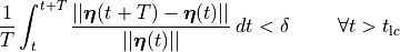
which would the relative difference between two cycles is, on average, less than a desired relative error .
Under this norm it is still possible that relative differences exceed
While using norms to detect the instant beyond which the state trajectories traverse a stable limit cycle
is certainly feasible, one has to keep in mind that various myocyte models will not arrive at a stable limit cycle
in the strict mathematical sense and that myocytes in vivo never operate in a regime
that would comply with such a rigorous constraint.
A more pragmatic approach is to determine by visual inspection.
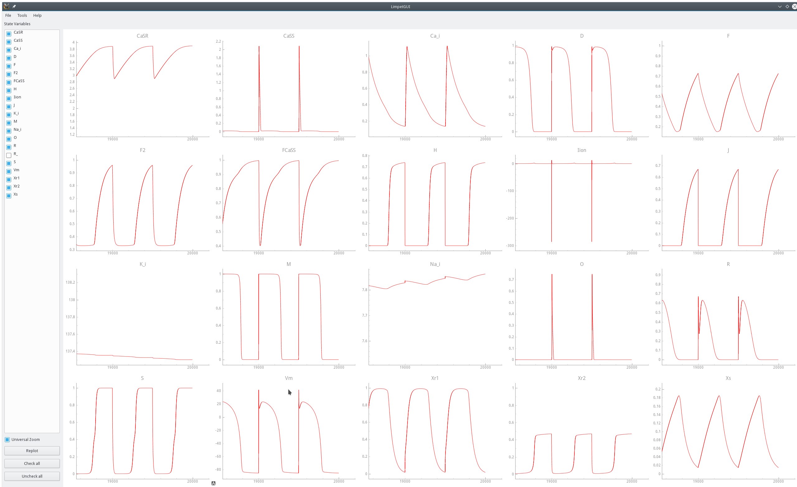
This is easily achieved with limpetGUI by pacing a cell for a sufficiently larger number of pacing cycles
and simply observe the envelope of all state time traces.
For the purpose of illustration an example is shown in fig-TT2-limit-cycle-envelope and fig-TT2-limit-cycle-zoom.
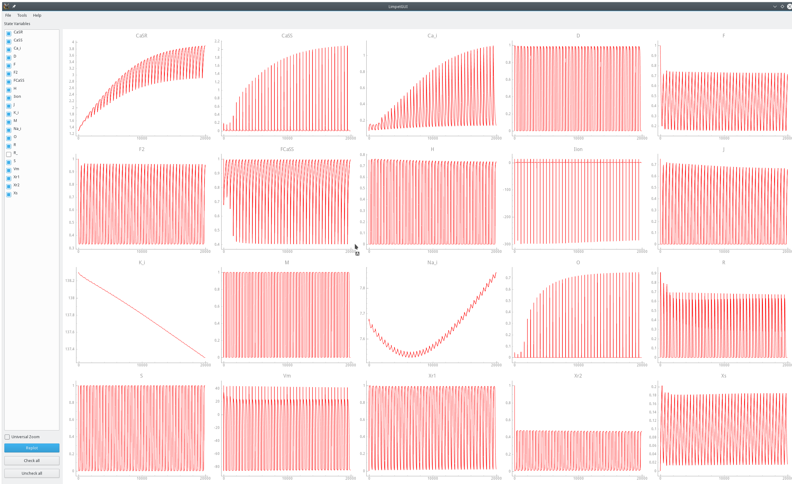
Visualization of a limit cycle pacing experiment using limpetGUI. After 20 seconds pacing at a bcl of 500 ms most state variables settle in at a limit cycle with the exception of intracellular concentration of sodium and potassium ions.
Zoom on state traces over the last three pacing cycles of the same pacing experiments shown above in fig-TT2-limit-cycle-envelope.
Initial state
Models of cellular dynamics are virtually never used with the values given for the initial state vector. Rather, cells are based to a given limit cycle to approximate the experimental conditions one is interested in. The state of the cell can be frozen at any given instant in time and this state can be reused then in subsequent simulations as initial state vector. Typically, the state of a cell is frozen in its limit cycle right at the end of the last diastolic interval. The standard procedure based on bench would proceed along the following steps:
Parameterize and augment a cell model corresponding to the experimental conditions of interest and for the intended application
Run bench then for a sufficiently large number of pacing pulses
numstimuntil a reasonable approximation of a stable limit cycle is achieved for the given cycle lengthbcl. Confirm the arrival at a limit cycle at least visually using limpetGUI.Store the initial state vector at the very end of the pacing protocol, that is, for
numstimstimuli and a givenbcldetermine the end time of the pacing protocol astsave = tstart + bcl*numstimSave the state vector at the determined time
tsaveinto a state vector file.
The last step of saving the state vector is triggered using the parameters --save-ini-time and --save-ini-file.
If we want to save the state of a myocyte after 25 pacing pulses at a basic cycle length of 500 ms
with the time of delivering the first pacing pulse at 0 ms one saves the initial state vector as follows:
# run baseline model
bench --imp TT2 --plug-in "LandHumanStress" --fout=TT2_baseline \
      --stim-start 0. --numstim 25 --bcl 500 --duration 12500 \
      --save-ini-time 12500 --save-ini-file TT2_lc_bcl_500_baseline.sv

# run modified PZ model
bench --imp TT2 --plug-in "LandHumanStress" --imp-par="GNa-62%,GCaL-69%,Gkr-70%,GK1-80%"  --fout=TT2_PZ \
      --stim-start 0. --numstim 25 --bcl 500 --duration 12500 \
      --save-ini-time 12500 --save-ini-file TT2_lc_bcl_500_PZ.sv
These runs generate two state vector files, TT2_lc_bcl_500_baseline.sv and TT2_lc_bcl_500_PZ.sv
which store the state of each state variable at the instant t=12500 ms under the above given pacing protocol.
For instance, the state vector under baseline conditions in the file TT2_lc_bcl_500_baseline.sv
will be similar to:
-85.2262            # Vm
1                   # Lambda
0                   # delLambda
0.308053            # Tension
-                   # K_e
-                   # Na_e
-                   # Ca_e
0.00256503          # Iion
-                   # tension_component
TT2
0.126796            # Ca_i
3.62845             # CaSR
0.000380231         # CaSS
0.907029            # R_
2.68967e-07         # O
7.62609             # Na_i
137.689             # K_i
0.00172638          # M
0.743346            # H
0.678447            # J
0.0150679           # Xr1
0.470865            # Xr2
0.0143382           # Xs
2.43132e-08         # R
0.999995            # S
3.3857e-05          # D
0.729795            # F
0.959628            # F2
0.995618            # FCaSS

LandHumanStress
0.0249847           # TRPN
0.999196            # TmBlocked
0.000641671         # XS
8.33073e-05         # XW
0                   # ZETAS
0                   # ZETAW
0                   # __Ca_i_local
Action Potential Duration (APD) Restitution Experiments
The single cell EP tool bench provides built-in capabilities for performing restitution experiments.
Restitution experiments with bench are steered through the following command line arguments
--restitute, --res-file and --res-trace.
--restitute
             pick the protocol for performing the restitution experiment.
             Possible values are "S1S2", "dyn" or "S1S2f".

--res-file
             definition file for restitution parameters.
             For a description of restitution file formats see :ref:`restitution protocol definition <restitution-protocol-def>`.
             By default no restitution protocol defintion file is provided.

--res-trace
             Can be on or off, toggles writing of trace files
Action potential analysis data are written in the following format:
#Beat Pre(P||*) lc  APD(n)  DI(n)   DI(n-1)  Tri   VmMax   VmMin

1     *          0  288.95  711.04   11.69   0.00  44.30  -86.08
2     *          0  286.97  713.02  711.04   0.00  45.27  -86.04
3     *          0  288.58  711.42  713.02   0.00  45.31  -86.01
4     *          0  304.53  695.00  711.42  78.29  45.37  -85.98
5     *          0  305.50  694.50  695.00  78.54  45.26  -85.95
6     *          0  305.90  694.10  694.50  78.74  45.31  -85.92
7     *          0  306.26  693.74  694.10  78.93  45.33  -85.90
8     *          0  306.59  693.40  693.74  79.11  45.20  -85.87
where the column headers refer to: #Beat - the total beat number in the protocol; Pre - whether beat was premature P or not ***; lc - whether AP traversed a limit cycle in the state space, 1, or not, 0; DI(n) - diastolic interval in ms of the current beat and DI(n-1) of the previous beat; Tri - Triangulation of the AP; VmMax and VmMin - maximum and minimum value of AP within pacing cycle.
Restitution data are written following the same format, but keeping only those beats which were marked as premature in the AP analysis file.
33    P          0  276.07  723.94  180.25  85.35  41.02  -85.58
46    P          0  272.73  727.27  170.63  85.93  40.11  -85.53
59    P          0  268.79  731.22  161.30  86.36  39.19  -85.49
72    P          0  264.53  735.47  151.97  86.84  38.27  -85.46
85    P          0  259.94  740.07  142.59  87.34  37.29  -85.43
98    P          0  255.01  744.99  133.16  87.94  36.20  -85.40
111   P          0  249.66  750.35  123.70  88.61  35.02  -85.37
124   P          0  243.87  756.14  114.14  89.45  33.68  -85.35
137   P          0  237.56  762.45  104.56  90.45  32.18  -85.32
150   P          0  230.68  769.32   94.94  91.71  30.47  -85.30
For an introduction into using bench as a tool for measuring restitution curves see the restitution experiments in the tutorials.
Tissue Scale
Model Equations
Discrete Representation
At a microscopic level cardiac tissue is a discrete structure
which is composed of myocytes interconnected
To understand activity at very fine resolutions, a discrete approach can be used where each cell is explicitly represented.
Ionic models of cells are connected to neighbouring cells with connectivity defined to represent actual tissue structure.
Gap junctions, providing the electrical coupling between cells, are depicted as ohmic resistances with the net cellular
membrane current,  , given as
()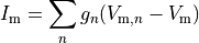
where  is the neighbourhood of cells connected by gap junctions,
 is the gap junctional conductance between the cell under consideration and neighbour
which has a transmembrane voltage
is the gap junctional conductance between the cell under consideration and neighbour
which has a transmembrane voltage  .
A positive value of will lead to cellular depolarization
which can trigger an action potential if strong enough.
This equation can be combined with Eqn.~ref{eqn:Imdef} to determine the time course of the voltage.
.
A positive value of will lead to cellular depolarization
which can trigger an action potential if strong enough.
This equation can be combined with Eqn.~ref{eqn:Imdef} to determine the time course of the voltage.
Homogenization
The number of myocytes in the human heart is estimated to be in the range 2–3 billion. As such, this makes explicitly representing every cell computationally intractable. Instead of a discrete representation of individual cells, cardiac tissue is represented as a continuum in which properties are averaged over space. Homogenization is the process of determining a homogeneous material property which best replicates behaviour of the heterogeneous domain. Homogenized cardiac domain properties must be derived by taking into account myoplasmic properties, cellular structure, connectivity and orientation changes. The process assumes that properties and structure are the same in the subdomain being homogenized, allowing an average representation to be used.
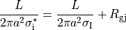
When determining homogenized conductivity values which encompass several myocytes,
there are two components to consider, one for the resistance of the cytoplasm, and one for the resistance of the gap junctions.
This is easily computed for the case of connected cylinders.
Considering the cylinders to have radius  and length
  with cytoplasmic conductivity
  and a gap junction resistance between cells of
  , we find the
homogenized conductivity
, we find the
homogenized conductivity  from the following equation:
()
The value of is itself homogenized
since cytoplasm has a conductivity close to that of sea water (1 S/m), but
the presence of organelles restrict the conduction path to decrease the effective conductivity.
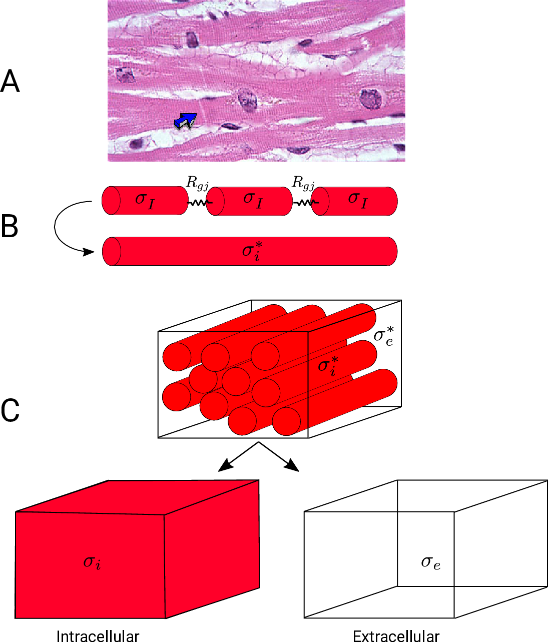
A: Histological section of cardiac tissue. Nuclei are seen as purple ovals.
Junctions between cells are visible and oone is highlighted by the blue arrow.
B: Discrete myocytes with intracellular conductivity
are represented as cylinders, connected by gap junctions of resistance  ,
and form a syncytium with an equivalent conductivity, .
C: In the bidomain representation, tissue is composed of myocytes surrounded by an extracellular space.
After homogenization, the original volume is considered as two coincident domains,
each with homogenized properties.
,
and form a syncytium with an equivalent conductivity, .
C: In the bidomain representation, tissue is composed of myocytes surrounded by an extracellular space.
After homogenization, the original volume is considered as two coincident domains,
each with homogenized properties.
A further homogenization is required for mathematical approaches which treat intracellular and extracellular spaces to be continuous and everywhere within the cardiac tissue. These approaches consider each point to be in both spaces which is physically impossible. In effect, both domains are rescaled to fill the entire domain. Continuing the example of myocytes as cylinders packed in a volume, the effective conductivity in the longitudinal direction becomes
()
where  is the portion of the surface area of a plane orthogonal to the longitudinal axis
which is intracellular space.
Parameter values used in simulations may be quite different
from experimentally measured specific material properties due to homogenization.
is the portion of the surface area of a plane orthogonal to the longitudinal axis
which is intracellular space.
Parameter values used in simulations may be quite different
from experimentally measured specific material properties due to homogenization.
Bidomain Equation
Two domains are preserved in the formulation, the extracellular or interstitial space comprising the volume outside of and between the cells, and the intracellular space within myocytes. The membrane separates the intracellular from interstitial space. Due to the high degree of coupling, the intracellular space is considered a functional syncytium. The bidomain equations result from assuming that intracellular and extracellular domains exist everywhere, and that current flows between them by crossing the separating membrane, resulting in the following equations:
()
where  and
and  are the electrical potential and homogenized conductivity
in the domain
are the electrical potential and homogenized conductivity
in the domain  respectively, where is
  or
or  for intracellular or extracellular.
The conductivity tensors describe the orthotropic eigendirections of the tissue at a given location,
for intracellular or extracellular.
The conductivity tensors describe the orthotropic eigendirections of the tissue at a given location,  ,
and are constructed as
,
and are constructed as
()
where  ,
,  and
and  are conductivities of the domain
along the local eigenaxes,
are conductivities of the domain
along the local eigenaxes,  , along the prevailing myocyte orientation referred to as fiber orientation,
perpendicular to the fiber orientation but within a sheet,
, along the prevailing myocyte orientation referred to as fiber orientation,
perpendicular to the fiber orientation but within a sheet,  , and the sheet normal direction,
  .
.
()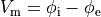
is the transmembrane voltage;
is the surface area of membrane contained within a unit volume;
 is an extracellular current density, specified on a per volume basis,
which serves as a stimulus to initiate propagation;
is an extracellular current density, specified on a per volume basis,
which serves as a stimulus to initiate propagation;
At tissue boundaries, no-flux boundary conditions are imposed on  and
and  , i.e.,
()
holds. In those cases where cardiac tissue is surrounded by a conductive medium, such as blood in the ventricular cavities or a perfusing saline solution, an additional Poisson equation has to be solved
()
where  is the isotropic conductivity of the conductive medium and
 is the stimulation current injected into the conductive medium.
In this case, no flux boundary conditions are assumed at the boundaries of
the conductive medium, whereas continuity of the normal component of the
extracellular current and continuity of are enforced at the
tissue-bath interface. That is,
is the stimulation current injected into the conductive medium.
In this case, no flux boundary conditions are assumed at the boundaries of
the conductive medium, whereas continuity of the normal component of the
extracellular current and continuity of are enforced at the
tissue-bath interface. That is,
()
The no-flux boundary condition for along the tissue-bath interface remains unchanged
as the intracellular space is sealed there.
Equations (ref{eq:bidm_i}-ref{eq:bidm_e}) are referred to as the parabolic-parabolic form
of the bidomain equations, however, the majority of solution schemes is based
on the elliptic-parabolic form which is found by adding Eqs.~eqref{eq:bidm_i} and eqref{eq:bidm_e}
and replacing is by  .
This yields
.
This yields
()¶![\begin{eqnarray}
\left[
\begin{array}{c}
{ -\nabla \cdot \left( \boldsymbol{\sigma}_{\mathrm i} + \boldsymbol{\sigma}_{\mathrm e} \right) \nabla \phi_{\mathrm e} } \\
{ -\nabla \cdot \sigma_{\mathrm b} \nabla \phi_{\mathrm e} }
\end{array}
\right] &=&
\left[
\begin{array}{c}
{ \nabla \cdot \boldsymbol{\sigma}_{i} \nabla V_{\mathrm m} } \\
{ I_{\mathrm e} }
\end{array}
\right] \nonumber \\
-\left( \nabla \cdot \boldsymbol{\sigma}_{\mathrm i} \nabla V_{\mathrm m}
+\nabla \cdot \boldsymbol{\sigma}_{\mathrm i} \nabla \phi_{\mathrm e} \right) &=&
-\beta C_{\mathrm m} \frac{\partial V_{\mathrm m}}{\partial t} - \beta \left( I_{\mathrm {ion}} - I_{\mathrm {tr}} \right), \nonumber
\end{eqnarray}](_images/math/bdc1a8f8ca7141943e3a0d6fac9acea34045a24a.png)
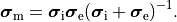
where and , the quantities of primary concern, are retained as
the independent variables. Note that Eq.~eqref{equ:Elliptic} treats the bath
as an an extension of the interstitial space.
Monodomain Equation
A computationally less costly monodomain model can be derived from the bidomain model under the assumption
that intracellular and interstitial conductivity tensors can be related by
 .
In this scenario Eq.~eqref{eq:bidm_e} can be neglected
and the intracellular conductivity tensor in Eq.
.
In this scenario Eq.~eqref{eq:bidm_e} can be neglected
and the intracellular conductivity tensor in Eq. eq-Parabolic is replaced by the harmonic mean tensor,
 ,
,
()
That is, the monodomain equation is given by
()
where  is a transmembrane stimulus current,
a current which is introduced in the intracellular space and immediately removed from the extracellular space.
In this case, monodomain and bidomain formulations are equivalent in the sense
that both models yield the same conduction velocities along the principal axes
which, in turn, results in very similar activation patterns.
Minor deviations are expected when wavefronts are propagating in any other directions
which results in slightly different activation patterns.
is a transmembrane stimulus current,
a current which is introduced in the intracellular space and immediately removed from the extracellular space.
In this case, monodomain and bidomain formulations are equivalent in the sense
that both models yield the same conduction velocities along the principal axes
which, in turn, results in very similar activation patterns.
Minor deviations are expected when wavefronts are propagating in any other directions
which results in slightly different activation patterns.
This formulation has the advantage that it is computationally an order of magnitude of faster to solve than the bidomain formulation.
Though the equal anisotropy assumption is known to not hold, the approximation is reasonably accurate in situations
where extracellular fields are not imposed, which precludes its use for defibrillation studies.
Nevertheless, extracellular potentials can be recovered from the monodomain solution through the following:
()
Numerical details on discretization and solution of the bidomain equations were given previously in several studies [2] [3] [4].
Eikonal model
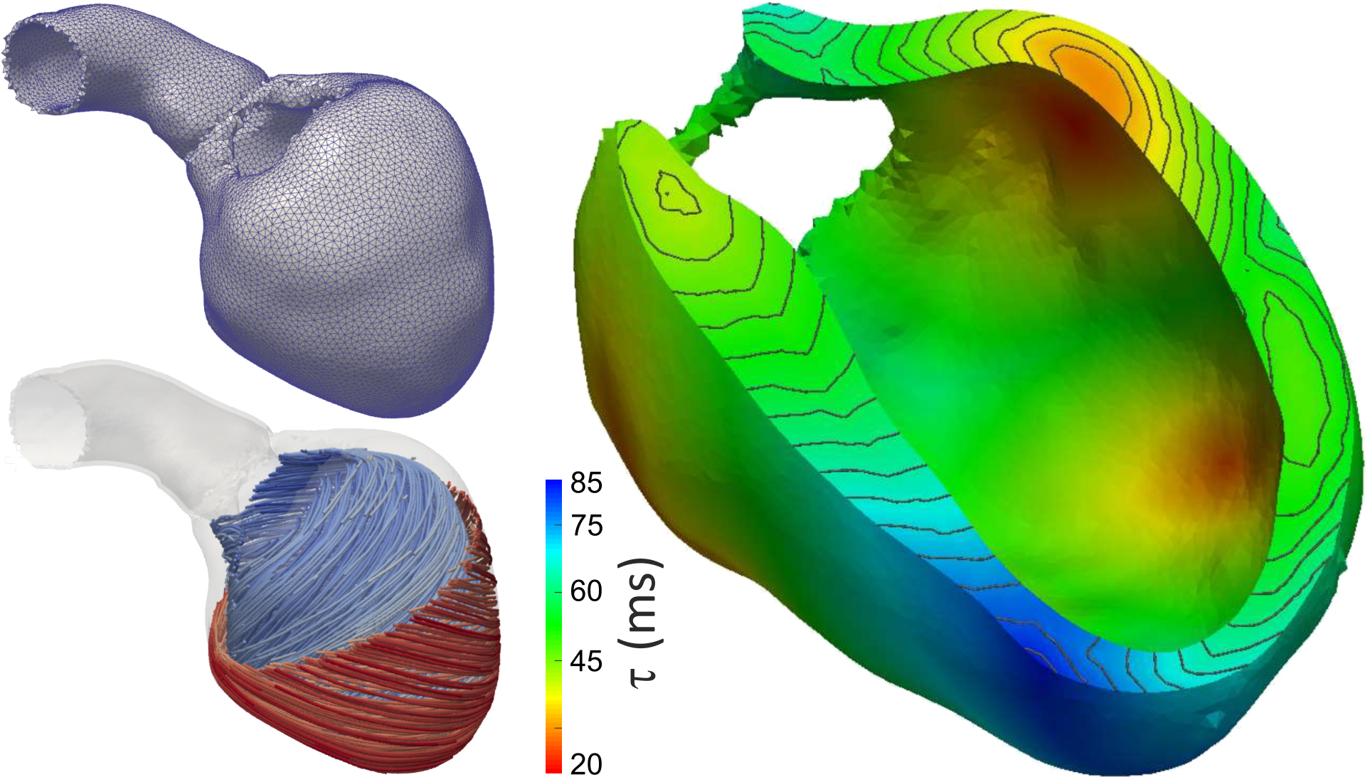
Shown is the solution of the eikonal curvature equation,  ,
(right panel) in a finite element mesh of the left ventricle (left top)
with anisotropic conduction properties (left bottom, streamlines indicate direction of fastest propagation).
,
(right panel) in a finite element mesh of the left ventricle (left top)
with anisotropic conduction properties (left bottom, streamlines indicate direction of fastest propagation).
Reaction-eikonal model
Electrical Stimulation
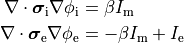
Basically, cardiac tissue can be stimulated either by changing the electrical potential
or by injection/withdrawal of currents.
In both cases stimulation can be applied in the intracellular domain,  ,
or in the extracellular domain,
,
or in the extracellular domain,  .
Mathematically, voltage stimuli correspond to Dirichlet boundary conditions
whereas current stimuli are implemented either as Neumann boundary condition
or, alternatively, as volume sources.
The choice of stimulation procedure should be based on the experimental conditions to be modelled
and the electronic circuitry used in the voltage/current source.
If stimulation is mediated via controlled injection of currents the current stimulation methods is preferible,
otherwise if voltage sources are used the voltage stimulation method should be used.
A special case is the stimulation with a transmembrane current
where current is injected in one domain and withdrawn in the other domain at the exact same location.
Thus the stimulus itself does not set up a primary extracellular field as there is no current path
between injecting and withdrawing electrode.
An introduction to using electrical stimulation in CARPentry is given in the
Extracellular Stimulation Tutorial.
.
Mathematically, voltage stimuli correspond to Dirichlet boundary conditions
whereas current stimuli are implemented either as Neumann boundary condition
or, alternatively, as volume sources.
The choice of stimulation procedure should be based on the experimental conditions to be modelled
and the electronic circuitry used in the voltage/current source.
If stimulation is mediated via controlled injection of currents the current stimulation methods is preferible,
otherwise if voltage sources are used the voltage stimulation method should be used.
A special case is the stimulation with a transmembrane current
where current is injected in one domain and withdrawn in the other domain at the exact same location.
Thus the stimulus itself does not set up a primary extracellular field as there is no current path
between injecting and withdrawing electrode.
An introduction to using electrical stimulation in CARPentry is given in the
Extracellular Stimulation Tutorial.
Extracellular voltage stimulation
Mathematically, intracellular voltage stimulation is easily feasible,
but since this is of very limited practical relevance support for this type of stimulation is not implemented.
Voltage stimulation is therefore always applied in the extracellular domain  .
This is achieved by applying Dirichlet boundary conditions in
which directly alter extracellular potentials.
If we consider the bidomain equation governing the extracellular potential field
.
This is achieved by applying Dirichlet boundary conditions in
which directly alter extracellular potentials.
If we consider the bidomain equation governing the extracellular potential field
()
or in the elliptic-parabolic cast given by
()
extracellular voltage stimulatin is achieved
by enforcing the extracellular potential  to follow a given time course,
i.e.the prescribed stimulus pulse shape, over the entire electrode surface,
to follow a given time course,
i.e.the prescribed stimulus pulse shape, over the entire electrode surface, 
()
or, alternatively, also a spatial variation of extracellular potentials  is possible, that is,
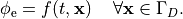
In practice, voltage stimulation is performed with voltage sources. Voltage sources have two terminals which impose a potential relative to a reference usually referred to as ground (GND). Often one terminal is grounded, i.e.connected to a zero potential, whereas the other terminal prescribes the time course of the chosen pulse shape. Many other variations are also possible, but not all will be discussed. In the following we restrict ourselves to configurations which are realized typically in stimulation circuits.
Extracellular voltage stimulation with GND
This is the default setup for modeling extracellular voltage stimulation
where one terminal of the voltage sources is used
to prescribe the time course of the extracellular potential at one electrode,
and enforce a zero potential at the corresponding electrode.
If the enforced potentials are positive, that is  holds,
the positive terminal acts as an anode and the grounded terminal acts as a cathode.
Such a configuration sets up an electric stimulation circuit as shown in
holds,
the positive terminal acts as an anode and the grounded terminal acts as a cathode.
Such a configuration sets up an electric stimulation circuit as shown in fig-extraV-wgnd.
On theoretical grounds, there is no necessity for using a ground electrode in this case
as a unique solution for the elliptic problem can be found by using one Dirichlet boundary conditions,
that is, using the electrode prescribing the stimulus pulse would suffice.
However, such a setup cannot be realized with an electric circuit and as such
it is unlikely to be suitable for matching a given experimental scenario.
Standard setup for extracellular voltage stimulation.
The positive terminal of the voltage source acts as an anode
by prescribing the time course of extracellular potentials .
The grounded electrode connected with the negative terminal of the voltage source acts as a cathode.
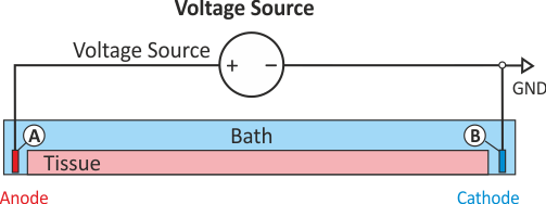
Symmetric extracellular stimulation with GND
The extracellular potential distribution  induced by the standard setup for extracellular voltage stimulation is not symmetric.
Under various circumstances it may be convenient to enforce an extracellular electric field
which is symmetric with regard to the two electrodes. Such a potential distribution can be enforced
using two electrodes of exactly opposite polarity and an additional ground
which then the zero potential isoline to run through the location of the grounding electrode.
This setup is shown in
induced by the standard setup for extracellular voltage stimulation is not symmetric.
Under various circumstances it may be convenient to enforce an extracellular electric field
which is symmetric with regard to the two electrodes. Such a potential distribution can be enforced
using two electrodes of exactly opposite polarity and an additional ground
which then the zero potential isoline to run through the location of the grounding electrode.
This setup is shown in fig-extraV-symm-wgnd.
Configuration details for this setup are found XXX.
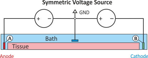
Setup for generating a symmetric extracellular potential field. Electrodes A and B impose the exact same time course of , but with inverted signs. The location of the GND electrode determines the location of the zero potential isoline.
Open versus closed circuit stimulation
Depending on a given hardware, a switch may or may not interrupt the circuit after pulse delivery.
If a switch remains closed for the entire simulation the potential at both electrodes
are governed by the potentials of the terminals of the voltage source.
Typically, the potential at both terminals will be zero after the pulse delivery, that is,
both electrodes act as GND.
This may not always be desired. If a switch interrupts the circuit after delivery
the potential at one terminal is allowed to float whereas the other terminal will act as ground.
An illustration of the difference between the two modes is given in fig-extraV-wgnd-switched.
Extracellular voltage stimulus with a switched terminal to interrupt the circuit after stimulation. In contrast to the standard setup for extracellular voltage stimulation the potential at electrode A is not clamped to a prescribed potential after the end of the pulse delivery, the potential there is allowed to float freely then.
Extracellular current stimulation
In many cases tissue is stimulated by injecting current through a current source. Modelingwise current stimulation is simpler to implement as there is no need for manipulating the left hand side of the equation system. Mathematically, current injection is modelled either as a Neumann boundary condition given as
()
or, alternatively, as a volmetric current source given as
()
where  is the volumetric current density.
While there are FEM-theoretical advantages of using a Neumann approach,
in terms of ease of implementation volumetric sources are more flexible and easier to handle.
A Neumann approach injects current through the surface of an electrode into the surrounding domain.
This is straight forward to implement when electrodes are located at the boundary of the extracellular domain
.
However, in many scenarios this is not the case, for instance, when modeling current injection into the blood pool of the RV
using a RV coil electrode of an implanted device.
In this case elements enclosed by the surface of the Neumann electrode should be removed.
The use of volumetric sources is simpler in this regard.
Electrodes can be located at arbitrary locations. The downside of volumetric sources is
that this method is not entirely mesh independent (current is injected via the FEM hat functions
and the total volume therefore varies therefore due to variability in the surface representation).
CARPentry implements volumetric sources, Neumann current sources are not implemented.
In those cases where mesh resolution dependence is unacceptable the total current to be injected can be prescribed
which is used for internal scaling of current density such that the prescribed total current is injected
indepdently of mesh resolution.
is the volumetric current density.
While there are FEM-theoretical advantages of using a Neumann approach,
in terms of ease of implementation volumetric sources are more flexible and easier to handle.
A Neumann approach injects current through the surface of an electrode into the surrounding domain.
This is straight forward to implement when electrodes are located at the boundary of the extracellular domain
.
However, in many scenarios this is not the case, for instance, when modeling current injection into the blood pool of the RV
using a RV coil electrode of an implanted device.
In this case elements enclosed by the surface of the Neumann electrode should be removed.
The use of volumetric sources is simpler in this regard.
Electrodes can be located at arbitrary locations. The downside of volumetric sources is
that this method is not entirely mesh independent (current is injected via the FEM hat functions
and the total volume therefore varies therefore due to variability in the surface representation).
CARPentry implements volumetric sources, Neumann current sources are not implemented.
In those cases where mesh resolution dependence is unacceptable the total current to be injected can be prescribed
which is used for internal scaling of current density such that the prescribed total current is injected
indepdently of mesh resolution.
It should be noted that the elliptic PDE as given in Eq. ()
which has to be solved to find the extracellular potential distribution  is a pure Neumann problem and as such is singular.
That is, the solution can only be determined up to a given constant
as the Nullspace of a scalar Neumann problem comprises all constant functions.
Without using a Dirichlet boundary condition the problem cannot be solved therefore
unless an additional equation is used to constrain the solution in a unique way.
An often used constraint is to enforce the average potential in the domain to be zero,
that is
is a pure Neumann problem and as such is singular.
That is, the solution can only be determined up to a given constant
as the Nullspace of a scalar Neumann problem comprises all constant functions.
Without using a Dirichlet boundary condition the problem cannot be solved therefore
unless an additional equation is used to constrain the solution in a unique way.
An often used constraint is to enforce the average potential in the domain to be zero,
that is
()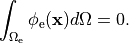
Such constraints can be imposed with various stabilization techniques.
Extracellular current stimulation with GND
The standard setup for extracellular current stimulation comprises an electrode for current injection
combined with a ground electrode.
The ground electrode enforces a homogeneous Dirichlet boundary
thus rendering the problem non-singular and solvable without any additional constraints.
As shown in fig-extraI-wGND, assuming the current source delivers a positive current pulse
current is being injected in electrode A thus lifting the extracellular potential there.
The increase in drives the transmembrane voltage towards more negative
values, thus electrode A hyperpolarizes tissue in its adjacency and acts therefore as an anodal stimulus.
Electrode B is grounded. Any current injected in A is automatically collected electrode B
without the need of explicitly withdrawing current there.
As current is withdrawn at electrode B, is being lowered there
which drives towards more positive values.
Thus electrode B depolarizes tissue in its adjacency and acts therefore as a cathodal stimulus.
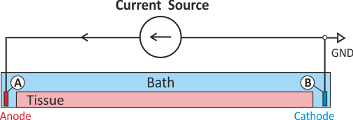
Shown is the standard setup for current stimulation. Current is injected through electrode A which acts as an anode hyperpolarizing tissue in its adjacency. Conversely, electrode B is used to withdraw current acting as a cathodal stimulus which depolarizes tissue in its adjacency.
Extracellular symmetric current stimulation with diffuse GND
Similar to the scenario described above, the standard setup for extracellular current stimulation does not generate a symmetric potential field. However, a symmetric potential field can be setup by using two current electrodes, for instance, electrode A is used for injection and electrode B for withdrawing currents. However, in this case an additional difficulty arises stemming from the fact that we attempt to solve a pure Neumann problem. There are a two things to keep in mind:
When solving a pure Neumann problem one has to comply with the compatibility condition which boils down to the fact that the sum of all currents injected and withdrawn must balance out to zero. If we integrate over Eqs we obtain
()
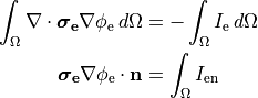
Using Gauss’ diverence theorem we obtain the compatibility condition
()

essentially meaning that all extracellular stimulus currents must add up to zero.
A pure Neumann problem can be solved without a Dirichlet condition by resorting to solver techniques which deal with the Nullspace of the problem. Typically, a condition such as Eq. () is enforced. This can be considered to be a diffuse floating ground (see Fig.
fig-extraI-symm-diffuse).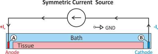
Shown is a stimulation setup using injection of extracellular currents which induces a symmetric extracellular potential field. Note that a pure Neumann problem is solved here. A diffuse ground is used to render the problem solvable which boils down to imposing the additional constraint that the mean extracellular potential
is zero (see Eq. ()).A setup with two current electrodes can be augmented with an additional reference electrode. In this case the compatibility condition does not need to be enforced. However, failure to balance the currents turns the ground electrode into an anode or cathode as any exess current will be collected by the ground electrode. Such a setup is shown in
fig-extraI-symm-wgnd.
Extracellular current injection with additional grounding electrode.
Definition of Electrical Stimuli
A complete definition of a stimulus comprises four components, the definition of electrode geometry, pulse shape, protocol and the physical nature of the pulse delivered (current or voltage). Stimuli are defined using the keyword stimulus[] where stimulus[] is an array of structures. The individual fields of the structure are defined in the following.
Geometry definition: Electrode geometries can be defined in two ways, indirectly by specifying a volume within which all mesh nodes are considered then to be part of this electrode, or, explicitly, by providing a vertex file containing the indices of all nodes to be stimulated.
The default definition is based on a block by specifying the lower left bottom corner and the lengths of the block along the Cartesian axes.
field type description name String Identifier for electrode used for output (optional) zd Float z-dimension of electrode volume yd Float y-dimension of electrode volume xd Float x-dimension of electrode volume z0 Float lower z-ordinate of electrode volume y0 Float lower y-ordinate of electrode volume x0 Float lower z-ordinate of electrode volume ctr_def flag if set, block limits are [ x0 - xd/2 x0 + xd/2], otherwise limits are [ x0 x0 + xd] etc Alternatively, other types of region than blocks are available such as spheres, cylinders or, the most general case, list of finite elements. See the definition of tag regions for details. Electrodes can be defined then by assigning the index of a tag region to the geometry field:
field type description geometry int Index of region pre-defined in tag region array tagreg[] An explicit definition of electrodes is also possible by providing a file holding all the mesh indices. A format definition of vertex files is given.
field type description vtx_file String File holding all nodal indices making up the electrode Pulse shape definition: By default, the pulse shape is defined as a monophasic pulse of square-like shape of a certain duration and strength. There are two time constants, one,
 , governs the leading and trailing edges of the pulse,
and one,
, governs the leading and trailing edges of the pulse,
and one,  , governs the plateau phase.
By default, these time constants are set to yield essentially a square-like pulse shape,
but can be easily adjusted to generate truncated exponential-like
pulses (see
, governs the plateau phase.
By default, these time constants are set to yield essentially a square-like pulse shape,
but can be easily adjusted to generate truncated exponential-like
pulses (see fig-pulse-shape-designfor details). Biphasic shapes are specified by two additional parameters, the duration of the first part of the pulse relative to the duration of the entire pulse (specified with![d1 \in (0,1]](_images/math/c91efb130d56f4f71a7a667de63eb2eac4f20a19.png) ),
and the strength of the second part of the pulse relative to the strength of the first part,
),
and the strength of the second part of the pulse relative to the strength of the first part,
![s2 \in [0,1]](_images/math/f630ea1c8b315ab3fea0bc9a1b3ab8c651ec492c.png) ).
The time constants for rising phases and plateau are the same for both polarities.
).
The time constants for rising phases and plateau are the same for both polarities.field type description s2 float strength relative to first part of biphasic pulse strength float amplitude of current ![[\mu A/cm^2]](_images/math/c4bcd2abcc30af0d226484def126538135a622a7.png) or voltage
or voltage ![[mV]](_images/math/afc8be4f1dc08ea0b1035ea02d14da386071b975.png)
total_current flag current strength is a total and not density d1 float duration of first part of biphasic pulse relative to total duration tau_edge float time constant for pulse edges tau_plateau float time constant for plateau bias float constant added to pulse duration float stimulus to be on pulse_file string Pulse file defining waveform 
balance int electrode with which to balance this electrode data_file string stimulus type-dependent data file An electrode balances another electrode be providing the same waveform as specified Electrode but of opposite polarity. For extracellular current injection, the strength takes into account Element sizes so that total current exiting one electrode enters the balanced electrode.
Mathematically, the pulses,
 , are defined:
()
![\begin{align}
P(t) & = B + \begin{cases}
S \left(1-e^{-t/\tau_{\mathrm {edge}}}\right) e^{-t/\tau_{\mathrm plateau}} & t\in [0,t'] \\
S_2 \left(1-e^{-(t-t')/\tau_{\mathrm edge}}\right) e^{-(t-t')/\tau_{\mathrm plateau}} & t\in (t',t''] \\
P(t'')e^{-(t-t'')/\tau_{edge}} & t \in(t'',D]
\end{cases} \nonumber
\end{align}](_images/math/26bbb0f92e8d7fde0ef825ec1a91cafa90cf1d7f.png)
where
()
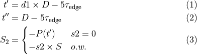
where
is the specified strength,  is the specified duration,
and
is the specified duration,
and  is the bias.
Note that for a monophasic pulse,
is the bias.
Note that for a monophasic pulse,  so that
  and only the top and bottom expressions are evaluated in Eq. ()}.
Note the following:
and only the top and bottom expressions are evaluated in Eq. ()}.
Note the following:- If
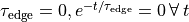 .
. - To get an exponentially rising pulse, set
 negative.
 - To get an identically constant value, set
 and
and  .
.
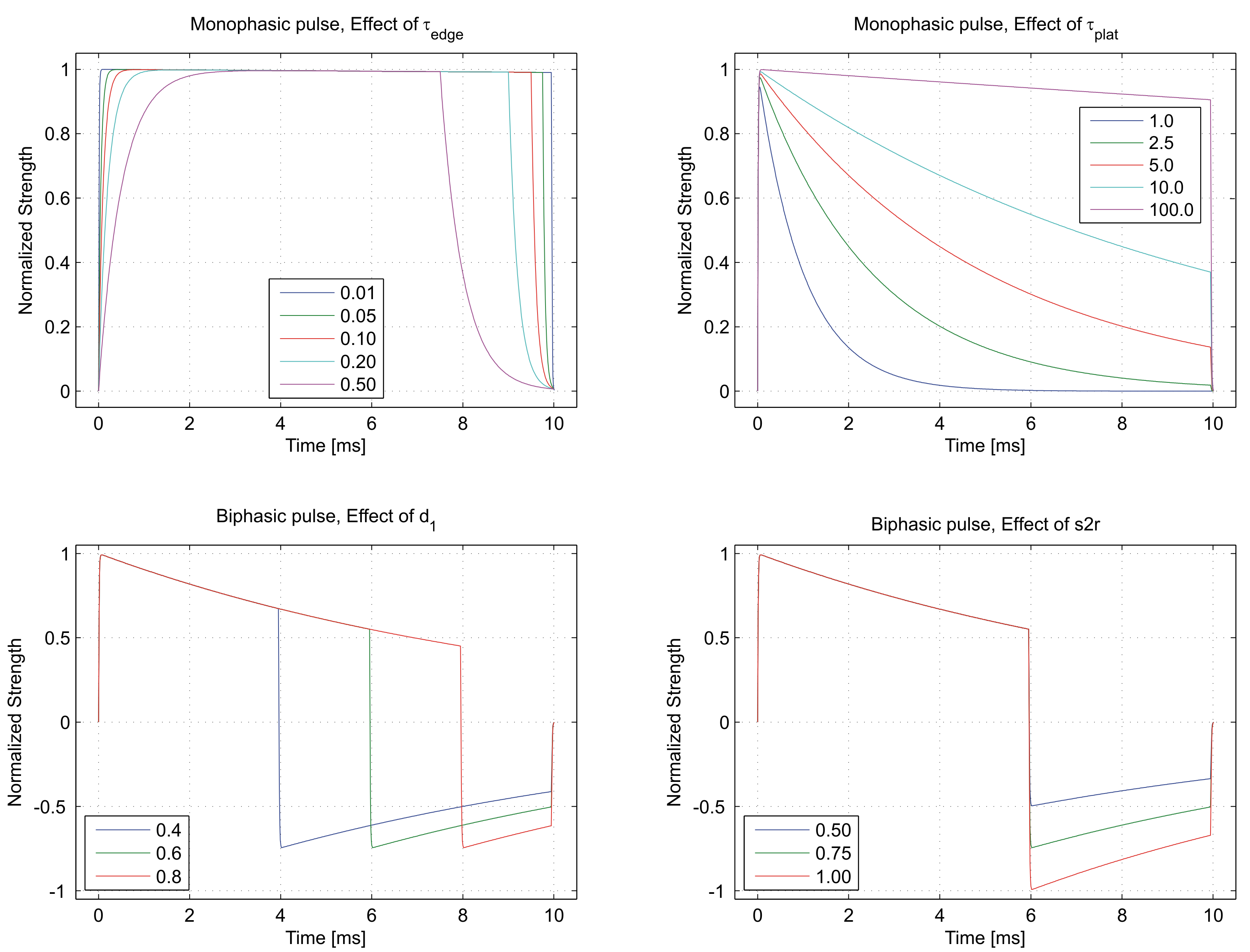
Top panels show the effect of parameters controlling the time constants of leading and falling edge
 ,
and the effect of the plateau time constant
,
and the effect of the plateau time constant  on a monophasic pulse.
Bottom panels show the effect of the duration ratio d1 and the strength ratio s2r
between the two phases of a biphasic stimulation pulse.
on a monophasic pulse.
Bottom panels show the effect of the duration ratio d1 and the strength ratio s2r
between the two phases of a biphasic stimulation pulse.- If
Stimulation source definition: The field stimtype field of the stimulus structure defines the physics of the actual source used for stimulating and, to some degree, also the wiring of the electric stimulation circuit. The following types of stimulation sources are supported:
field type value description stimtype short 0 transmembrane current 1 extracellular current 2 extracellular voltage (unswitched) 3 extracellular ground 4 intracellular current (unused) 5 extracellular voltage (switched) 6-7 unused 8 prescribed takeoff (see Reaction-eikonal model) 9 transmembrane voltage clamp Pacing protocol definition: The stimulus sequence is defined as a train of pulses. The number of pulses, the time interval between the pulses (pacing cycle length or basic cycle length) and the instant when first pulse is triggered defines the sequence in a unique manner. The following fields are used for the protocol definition:
field type description start float time at which stimulus sequence begins duration float duration of entire stimulus sequence npls int number of pulses forming the sequence (default is 1) bcl float basic cycle length for repetitive stimulation (npls > 1)
Electrical Tissue Properties
In CARPentry active and passive electrical tissue properties are assigned on a per region basis.
Regions are defined for a given properties as a set of tags (see Region Definition).
In cardiac electrophysiology simulations two distinct mechanisms are provided,
imp_region for the assignment of active electrophysiological properties,
that is, the assignment of models of cellular dynamics along with various specializations,
and gregion for the assignment of passive tissue properties
which govern subthreshold behavior and electrotonic features such as the space constant,  ,
but also influence suprathreshold phenomena such as conduction velocity and the spatial extent of depolarization wavefronts.
,
but also influence suprathreshold phenomena such as conduction velocity and the spatial extent of depolarization wavefronts.
Active Electrophysiological Properties
The number of regions is specified by num_regions.
Each region is preceded by imp_region[Int].
By default, elements are assigned {imp_region[0].
The following fields may be assigned:
| Variable | Type | Description |
|---|---|---|
| name | String | Region identification |
| num_IDs | Int | number of tags in the element file which belong to this regions |
| ID[Int] | Int * | array of the element tags belonging to the region |
| im | String | ionic model for this region. LIMPET specification |
| im_param | String | A comma separated list of parameters modifying the ionic model. These modifications are of the form param[=|*|/|+|-] float [%]. See the LIMPET library documentation for more details. |
| im_sv_dumps | String | comma separated list of state variables to dump from this IMP |
| im_sv_init | String | A file containing the initial values for variables’ statelabel{imsvdump} |
| plugins | String | comma separated list of plug-ins to use with the ionic model |
| plug_param | String | A colon separated list of comma separated lists specifying the plug-in parameters to modify. These are specified in the same order as the plug-ins are defined. |
| plug_sv_dumps | String | A colon list of comma separated lists specifying the state variables to dump for the plug-ins. Again, order must correspond to the order in which the plug-ins were specified. |
| cellSurfVolRatio | Float | If the ionic model does not specify the cellular surface to volume ratio, use this |
| volFrac | Float | fraction of tissue volume occupied by the cells |
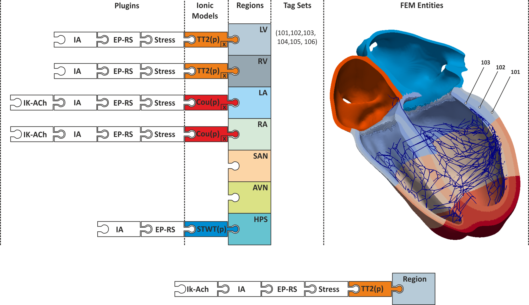
Conceptual view on defining regions of different electrophysiological properties.
A region of similiar electrophysiological properties is an imp_region.
Each region is defined based on a set of tags which refer to finite element entities,
typically nodes or elements. Each imp_region is assigned exactly one model of cellular dynamics.
The model is parameterized with a set of parameters,  , which are constant over the entire imp_region.
If necessary, parameters can also vary as a function of space, ,
using the ion_adjustment mechanism.
Each ionic model can be augmented dynamically with a number of plug-ins (see augmentation).
, which are constant over the entire imp_region.
If necessary, parameters can also vary as a function of space, ,
using the ion_adjustment mechanism.
Each ionic model can be augmented dynamically with a number of plug-ins (see augmentation).
Passive Electrophysiological Properties
Similarly, different conductivities may be assigned to different elements.
The number of conductivities is specified with num_gregions.
The conductivity regions are specified by gregion[Int].
with each element initially assigned to gregion[0] by default.
The following fields specify a conductivity region:
| Variable | Type | Description |
|---|---|---|
| name | String | Region identification |
| num_IDs | Int | number of tags in the element file which belong to this regions |
| ID[Int] | Int * | array of the element tags belonging to the region |
| g_et | Float | extracellular transverse conductivity |
| g_it | Float | intracellular transverse conductivity |
| g_el | Float | extracellular longitudinal conductivity |
| g_il | Float | intracellular longitudinal conductivity |
| g_en | Float | extracellular sheet normal conductivity |
| g_in | Float | intracellular sheet normal conductivity |
| g_bath | Float | isotropic bath conductivity |
| g_mult | Float | multiplicator for conductivity scaling of a gregion |
where  are conductivities in the intracellular domain along the axes
 ,
,  are the respective conductivities in the extracellular domain
and
are the respective conductivities in the extracellular domain
and  is an isotropic conductivity assigned to elements in this regions marked as bath.
Bath elements in a region which are marked to be anisotropic use the values.
is an isotropic conductivity assigned to elements in this regions marked as bath.
Bath elements in a region which are marked to be anisotropic use the values.
Discrimination between isotropic bath and anisotropic bath, that is, anisotropic non-myocardium as it would be appropriate for skeletal muscles, occurs when reading in a mesh. The difference between these two cases manifests in the element and fiber files. An isotropic bath element is described as
Element                   Fiber
ID [Node Indices] Tag     l
...
Tt  0 1 144 1226   2      0.0 0.0 0.0
...
That is, these elements are identified as having a zero fiber orientation vector
whereas anisotropic bath elements do have a preferred fiber vector, optionally also a sheet vector,
but the Tag in the element file is negative:
Element                   Fiber
ID [Node Indices] Tag     l
...
Tt  0 1 144 1226  -2      1.0 0.0 0.0
...
Electrical Mapping
Measuring Reference Time Markers
The main purpose here is to detect at which instants in time
nodes are activated in the tissue. These instants are usually referred to
as local activation times. Experimentally, this is done usually
using extracellular signals, as input,
but transmembrane voltages can also be used, for instance,
when glass micro-electrodes are used (which would actually measure )
or in optical mapping experiments where  (see Sec. Optical Mapping is measured which is considered a surrogate for .
The implementation of this feature is actually more general,
it is an event detector that records the instants when the selected event type occurs.
Local activation detection in the extracellular signals usually relies on
detecting the minimum of the derivative of , i.e.  .
One could also detect the maximum of the derivative of , or,
the crossing of the action potential with a given threshold
which has to be chosen larger than the threshold for sodium activation.
That is, with one picks the maximum of
.
One could also detect the maximum of the derivative of , or,
the crossing of the action potential with a given threshold
which has to be chosen larger than the threshold for sodium activation.
That is, with one picks the maximum of  or when crosses the prescribed threshold with a positive slope.
Equally, one could look for crossing of with a negative slope
to detect repolarisation events. The basic idea is outlined in
or when crosses the prescribed threshold with a positive slope.
Equally, one could look for crossing of with a negative slope
to detect repolarisation events. The basic idea is outlined in fig-lats-detection.
There can be num_LATs measurements and activation
can be defined in terms of a threshold or a derivative.
The activation measurements are named lats[Int].
with the following fields:
| field | type | description |
|---|---|---|
| measurand | Int | what to measure. 0=voltage, 1=extracellular potential |
| all | Int | If set, will output all activations as they occur. If zero, only the first activation of each vertex will be output. When all points are activated, one file with all the LATs will be written. |
| method | Int | How to determine activation. If method==0, use the
time at which the threshold was crossed. If method==1,
use the time of maximum derivative. |
| mode | Flag | If method==0, look for threshold crossing
with a negative slope (positive slope is default),
if method==1, look for minimum derivative instead of maximum |
| threshold | Float | The threshold value for determining activation.
If method==0, this is the threshold for detecting
activation, if method==1 the threshold is used
to exclude small peaks in the derivative which are not considered
to be due to local activation. |
| ID | Wfile | output file name |
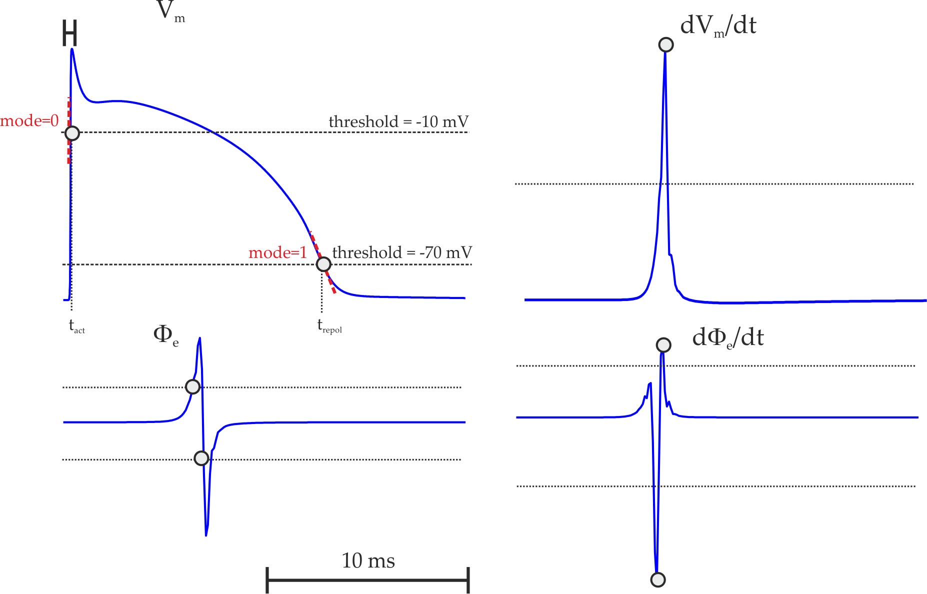
Illustration of using the lat detection feature:
a) With measurand ,
using method==0, threshold  and
and mode==0,
all positive slope intersections of with the given threshold are detected.
In this case the instant of local activation,  is detected.
Using threshold
is detected.
Using threshold  and
and mode==1 the negative slope intersections are detected
which could be used in this case for detecting a reference marker for the instant of repolarisation,  .
b) Using
.
b) Using method==1 with measurand==0 ()
detects the peak derivative of .
Any peak derivatives below a chosen threshold are ignored.
c) Using threshold crossing detection on the extracellular signal ,
i.e. measurand==1.
d) Using peak derivative detection on the extracellular signal  ,
i.e.
,
i.e. measurand==1 and mode==1.
A tutorial on how to use these features is found in the Electrical Mapping Tutorial.
Measuring Conduction Velocities
Explain carputils velocity script.
Cardiac Mechanics Modeling
Models of cardiac electromechanics (EM) comprise an electrophysiological and a mechanical component. Electrophysiology is represented by the bidomain equation or simplified derivations and mechanical deformation is described by Cauchy’s equation of motion. In the most general case the two PDE’s are coupled through excitation-contraction coupling (ECC) to translate electrophysiological activity into the buildup of active mechanical stresses, and mechano-electric feedback (MEF) by which the electrophysiological state of the tissue is altered by deformation. The full coupled system is given then by the bidomain equation in its deformed configuation
()¶![\begin{align}
%
\operatorname{Div}\left[J\mathbf{F}^{-1} \left( \boldsymbol{\sigma}_{\mathrm{i}} + \boldsymbol{\sigma}_{\mathrm{e}} \right) \mathbf{F}^{-\top}\nabla\, \phi_{\mathrm{e}}\right]
&= -\operatorname{Div}\left[J \mathbf{F}^{-1} \boldsymbol{\sigma}_{\mathrm{i}} \, \mathbf{F}^{-\top}\nabla V_{\mathrm{m}}\right] -I_{\rm e} \nonumber \\
%
\operatorname{Div}\left[J\mathbf{F}^{-1} \boldsymbol{\sigma}_{\mathrm{i}} \, \mathbf{F}^{-\top} \nabla V_{\mathrm{m}}\right]&=
-\operatorname{Div}\left[J\mathbf{F}^{-1} \boldsymbol{\sigma}_{\mathrm{i}} \, \mathbf{F}^{-\top}\nabla\phi_{\mathrm{e}} \right]
+ \beta \left( I_{\mathrm{m}} - I_{\mathrm{tr}} \right), \nonumber \\
I_m &= C_m \frac{\partial V_m}{\partial t} + I_{\text{ion}}(V_m,\boldsymbol{\eta}_{\rm e},\lambda) \nonumber \\
V_m &= \Phi_i - \Phi_e \nonumber \\
\frac{\partial \boldsymbol{\eta}_{\rm e}} {\partial t} &= f(V_{\rm m}, \boldsymbol{\eta}_{\rm e}, [Ca^{2+}]_{\rm i}(\lambda),\lambda), \nonumber
\end{align}](_images/math/33ac68487322cd8c7e29f4e3322e00d31df1c8f4.png)
and Cauchy’s equation of motion cast in the so-called Lagrange configuration given as
()¶![\begin{eqnarray}
-\operatorname{Div}\left[ \mathbf{F}\mathbf{S}(\mathbf{u})\right] &=& \mathbf{b}_0
\quad \mbox{ in} \quad \Omega_0 \nonumber \\
\mathbf{S} &=& \mathbf{S}_\mathrm{p}+ \mathbf{S}_\mathrm{a} \nonumber \\
\mathbf{S}_{\mathrm{p}} &=& 2 \frac{\partial \Psi(\mathbf{C})}{\partial \mathbf{C}} \nonumber \\
\mathbf{S}_{\mathrm{a}} &=& \sigma_{\rm a}\left(\mathbf{f}_0^\top\mathbf{C}\mathbf{f}_0\right)^{-1}\mathbf{f}_0 \otimes \mathbf{f}_0 \nonumber \\
\sigma_{\rm a} &=& f(\boldsymbol{\eta}_{\rm m}, [Ca^{2+}]_{\rm i}, [Ca^{2+}]_{\rm TnC}, \lambda,\dot{\lambda}) \nonumber \\
\lambda &=& \sqrt{\mathbf{f}_0^\top \mathbf{C} \mathbf{f}_0} \nonumber \\
\mathbf{u}&=&\mathbf{u}_{\mathrm{D},0}\quad\mbox{ on } \Gamma_{\mathrm{D},0} \nonumber \\
\mathbf{F}\mathbf{S}\mathbf{n}_0&=&-p J {\bf F}^{-\top}\mathbf{n}_0\quad\mbox{ on } \Gamma_{\mathrm{N},0} \nonumber
\end{eqnarray}](_images/math/96cc09f70ba35b7eaa4144996eef16ac6783ebed.png)
The physiology of EP is coupled to deformation through excitation-contraction coupling (ECC). During an action potential Calcium is released from intracellular stores inducing a rise in intracellular Calcium concentration
EP is influenced by deformation as well through mechano-electric feedback (MEF).
This is mainly driven by length-dependence of Calcium binding and stretch-activated sacrolemnal currents,
 , which modulated their conductivity as a function of fiber stretch, .
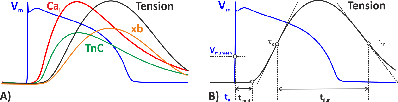
ECC mechanisms as implemented in carpentry. A) Physiological Calcium-based coupling mechanism: The upstroke of the action potential
triggers Calcium release from intracellular Calcium stores, thus driving the Calcium concentration up in the cytosol.
Calcium binds to Troponin C and mediates the formation of force-generating cross-bridges, xb, in myofilaments,
that leads then to the buildup of mechanical forces shortening the myocyte. Calcium is being pumped back into the intracellular stores
through the SERCA pump or removed from the cell through the sodium-Calcium exchanger current, .
B) Phenomenological active stress models are triggered based on a prescribed activation time. In carpentry
the instant of triggering is derived from the upstroke of the AP after a given delay,  ,
the electro-mechanical delay (which is fixed in this case and not a function of activation time as it would be in the physiological
case). The shape of the phenomenological tension transient can be matched to fit experimental measurements,
by adjusting parameters such as the rate of contraction,
,
the electro-mechanical delay (which is fixed in this case and not a function of activation time as it would be in the physiological
case). The shape of the phenomenological tension transient can be matched to fit experimental measurements,
by adjusting parameters such as the rate of contraction,  or relaxation,
  ,
the peak tension developed and the duration of the force twitch,
,
the peak tension developed and the duration of the force twitch,  .
.
Single Cell Scale
For coupling between EP and deformation three distinct cellular mechanisms are implemented which are chosen on the fly depending on the myofilament chosen.
Activation-based coupling with phenomenological myofilament models
These myofilament models trigger a twitch force transients depending on a prescribed instant of activation. Explicit prescription of activation times is not implemented in CARPentry, rather the instant of activation is derived from the upstroke of the action potential of the cell model. For instance
Calcium-based weak coupling with biophysical active stress models
In this scenario the active stress plugin is driven by the intracellular Calcium trace
 . As myocyte and myofilament are weakly unidirectionally coupled,
any effects due to stretch onto Calcium are ignored.
That is, enforcing a step change in length does not change intracellular Calcium
by binding more or less Calcium to the Troponin-C buffer.
That is, length and velocity dependence are accounted for, but not their feedback
on the electrophysiological state.
. As myocyte and myofilament are weakly unidirectionally coupled,
any effects due to stretch onto Calcium are ignored.
That is, enforcing a step change in length does not change intracellular Calcium
by binding more or less Calcium to the Troponin-C buffer.
That is, length and velocity dependence are accounted for, but not their feedback
on the electrophysiological state.
Calcium-based weak coupling with biophysical active stress models
In this scenario myocyte and myofilament model are strongly bidirectionally coupled, that is, enforcing a step change in length does change intracellular Calcium by binding more or less Calcium to the Troponin-C buffer.
A tutorial on how to configure single cell electromechanics is found here.
Excitation-Contraction Coupling (ECC)
At the single cell scale ECC and MEF mechanisms are steered through turning on specific plugins which account for
Essentially, there are three ways of how models of cellular dynamics can be coupled with active stress models:
- The easiest
Mechano-electric Feedback (MEF)
Tissue Scale
Passive Material Models
Holzapfel and Ogden (2009) myocardial model
The ventricular myocardium model
is a non-linear, hyperelastic, nearly incompressible and orthotropic material
with a layered organization of myocytes and collagen fibers that is
characterized by a right-handed orthonormal set of basis vectors.
These basis vectors consist of the fiber axis  , which
coincides with the orientation of the myocytes, the sheet axis
, which
coincides with the orientation of the myocytes, the sheet axis  and the sheet-normal axis
  .
.
Comparing to experimental data Holzapfel and Ogden reduced a constitutive law with the full set of invariants to a simplified model which combines the volumetric part, an isotropic Demiray part, two fiber parts and one fiber interaction part:
![\Psi(\boldsymbol{C}) = \frac{\kappa}{2}\ln(J)^2 + \frac{a}{2b}
\left\{ \exp\left[b(\overline{I}_1-3)\right]-1 \right\}
+ \sum_{i=\mathrm{f,s}} \left[\frac{a_i}{2b_i}\left\{\exp\left[b_i
(\overline{I}_i-1)^2\right]-1\right\}\right]
+ \frac{a_\mathrm{fs}}{2b_\mathrm{fs}}
\left\{ \exp\left[b_\mathrm{fs}\overline{I}_\mathrm{fs}^2\right]-1 \right\}](_images/math/b9e03810a8799b5435ae03e282afd1cd05453806.png)
with invariants
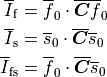
and parameters
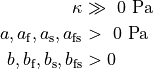
The default parameters are
| a | b | a_f | b_f | a_s | b_s | a_fs | b_fs | kappa | Data |
|---|---|---|---|---|---|---|---|---|---|
| 0.345 | 9.242 | 18.54 | 15.97 | 2.564 | 10.45 | 0.417 | 11.60 | 1000 | Dog |
Guccione et al. myocardial model
The passive behavior of myocardial tissue is modeled by a
nearly-incompressible, transversely isotropic Fung-type constitutive law,
first described by Guccione1991Passive and later also by
Costa1996Three.
The layered organization of myocytes and collagen fibers in the myocardium is
characterized by a right-handed orthonormal set of basis vectors consisting of
the fiber axis , which coincides with the orientation of the
myocytes, the sheet axis and the sheet-normal axis
.
The strain-energy function is given by
![\Psi(\boldsymbol{C})
= \frac{\kappa}{2} \left( \log\,J \right)^2
+ \frac{a}{2}\left[\exp(\overline{Q})-1\right],](_images/math/f91da6901a55a8ab912cc986ebb62b9d64b062fe.png)
where

and

with 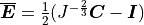 the modified isochoric Green–Lagrange strain tensor.
The bulk modulus
the modified isochoric Green–Lagrange strain tensor.
The bulk modulus  serves as a penalty parameter to
enforce nearly incompressibility and
serves as a penalty parameter to
enforce nearly incompressibility and  is a stress-like scaling
parameter. All other parameters
is a stress-like scaling
parameter. All other parameters 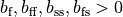 are dimensionless and negative values are not physically
acceptable. Default parameters are:
are dimensionless and negative values are not physically
acceptable. Default parameters are:
| a | b_ff | b_ss | b_nn | b_fs | b_fn | b_ns | kappa | Data |
|---|---|---|---|---|---|---|---|---|
| 0.876 | 18.48 | 3.58 | 3.58 | 3.58 | 1.627 | 1.627 | 1000 | Dog |
and were fitted to produce epicardial strains that were measured previously in the potassium-arrested dog heart.
Several modifications of the original model were published, most notably the simplified version due to Omens1993Measurement and Guccione1995Finite

This is also the version that is implemented in CARP. The parameters are then reduced to:
| a | b_ff | b_ss | b_fs | kappa | Data |
|---|---|---|---|---|---|
| 0.876 | 18.48 | 3.58 | 1.627 | 1000 | Dog |
Mechanical Boundary Conditions
The definition of mechanical boundary conditions follows the same basic concept as is used for defining electrical stimuli. First, a region of the mesh is defined, typically a set of surface nodes or faces, to which boundary conditions are applied. Subsequently, the quantity to apply and its time course is defined. These quantities in mechanics simulations are either a scalar pressure (Neummann boundary conditions), or vector displacements (Dirichlet boundary conditions).
The definition of mechanical boundary conditions uses an analog approach to the definition of electrical stimuli.
A complete definition of a mechanical boundary condition comprises two components,
the definition of the boundary (in terms of vertices or surface elements)
and the loading protocol.
Mechanical loading protocols are described as time traces
describing the time course of applied (scalar) pressure in the case of Neumann boundary conditions
or (vectorial) displacements in the case of Dirichlet boundary conditions.
The definition of Neumann and Dirichlet boundary conditions is very similar
with the major difference being the use of the keyword mechanic_nbc[]
for Dirichlet boundaries,
and mechanic_nbc[] for Neumann boundaries.
Geometry definition: Boundary geometries can be defined in two ways, indirectly by specifying a volume within which all mesh nodes are considered then to be part of this boundary, or, explicitly, by providing a surface file containing all surface elements spanning the boundary.
The default definition is based on a block by specifying the lower left bottom corner and the lengths of the block along the Cartesian axes.
| field | type | description |
|---|---|---|
| name | String | Identifier for electrode used for output (optional) |
| zd | Float | z-dimension of electrode volume |
| yd | Float | y-dimension of electrode volume |
| xd | Float | x-dimension of electrode volume |
| z0 | Float | lower z-ordinate of electrode volume |
| y0 | Float | lower y-ordinate of electrode volume |
| x0 | Float | lower z-ordinate of electrode volume |
| ctr_def | flag | if set, block limits are [ x0 - xd/2 x0 + xd/2], othewise limits are [ x0 x0 + xd] etc |
Alternatively, other types of region than blocks are available such as spheres, cylinders or, the most general case, list of finite elements. See the definition of tag regions for details. Electrodes can be defined then by assigning the index of a tag region to the geometry field:
| field | type | description |
|---|---|---|
| geometry | int | Index of region pre-defined in tag region array tagreg[] |
An explicit definition of boundary conditions is also possible by providing a file holding the defining mesh entities. Here the formats between Neumann and Dirichlet boundaries is different, see below.
| field | type | description |
|---|---|---|
| vtx_file | String | File holding all nodal indices making up the boundary |
| field | type | description |
|---|---|---|
| surf_file | String | File holding all surface elements making up the boundary |
Neumann Boundary Conditions
The definition of loading protocols differs between Neumann and Dirichlet boundaries due to the different physical quantities applied to the boundaries, i.e. scalar pressures always acting perpendicular to the Neumann boundary and vectorial displacement which can be enforced in any direction.
The Neumann loading protocol is defined based on two components, the time course of the applied load as defined in a trace file, and the magnitude of the load. Splitting of these two components offers the advantage of avoiding the redefinition of time traces for different magnitudes of loads.
Loading protocol definition: In the case of Neumann boundary conditions
the time course and magnitude of applied pressures must be defined
using the keywords summarized in tab-neumann-protocol-def.
| field | type | description |
|---|---|---|
| pressure | Float | pressure imposed on boundary in [kPa] |
| trace | File | trace file describing the time course of pressure |
Dirichlet Boundary Conditions
Loading protocol definition: In the case of Dirichlet boundary conditions
the time course and magnitude of applied displacements must be defined
using the keywords summarized in tab-neumann-protocol-def.
| field | type | description |
|---|---|---|
| ux | Float | rate of displacement along x in [ ] ] |
| uy | Float | rate of displacement along y in [] |
| uz | Float | rate of displacement along z in [] |
| ux_file | File | trace file describing time course of displacement ux |
| uy_file | File | trace file describing time course of displacement uy |
| uz_file | File | trace file describing time course of displacement uz |
| apply_ux | Flag | flag whether ux displacements are applied or not |
| apply_uy | Flag | flag whether uy displacements are applied or not |
| apply_uz | Flag | flag whether uz displacements are applied or not |
In the Dirichlet case the definition of repetitive loading is also support. The definition follows analog to the definition of electrical stimulation protocols, re-using the same terminology, that is, a single sequence is referred to as a pulse and the duration of a single sequence is referred to as pacing cycle length or basic cycle length.
| field | type | description |
|---|---|---|
| start | float | time at which Dirichlet loading sequence begins |
| duration | float | duration of entire Dirichlet loading sequence |
| npls | int | number of pulses forming the sequence (default is 1) |
| bcl | float | basic cycle length for repetitive stimulation (npls > 1) |
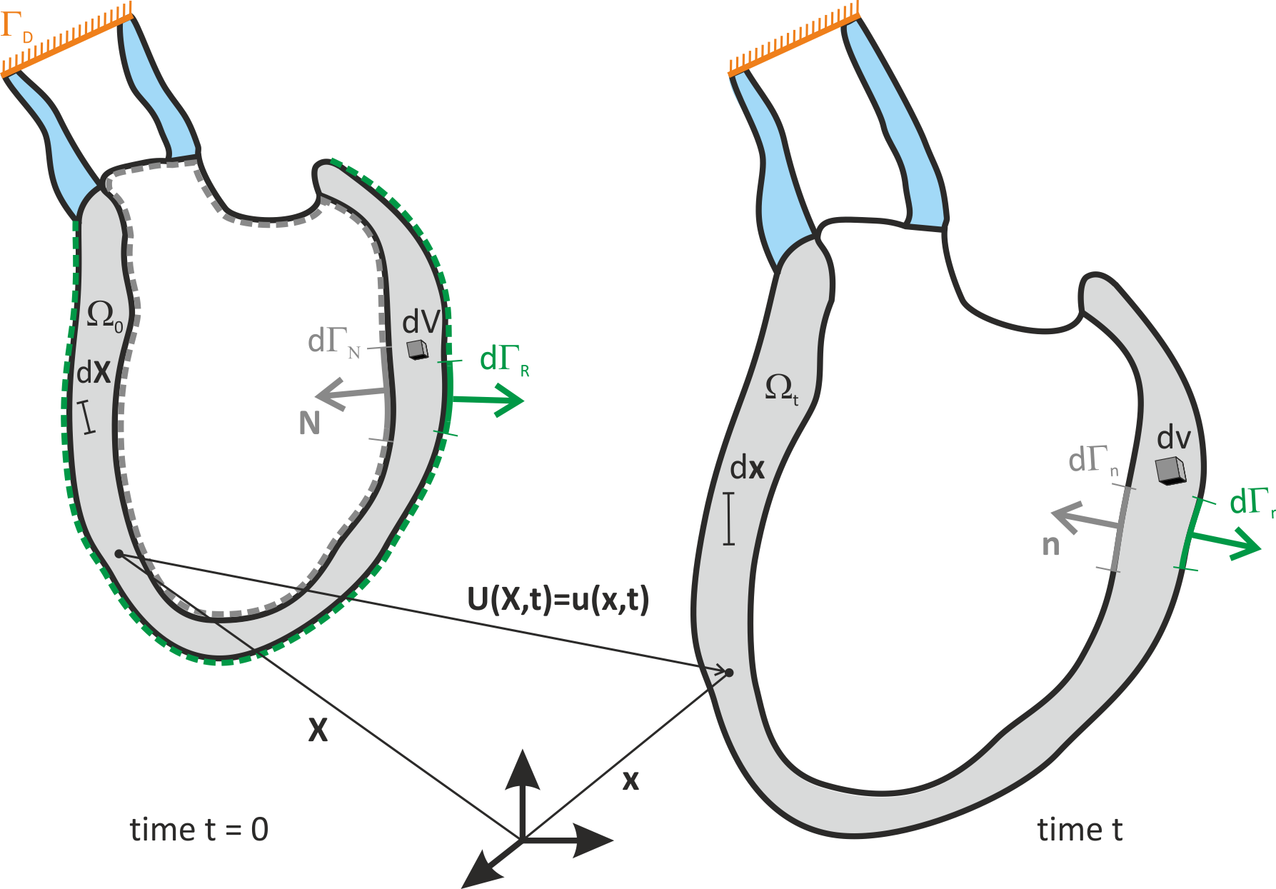
Deformation of an elastic body  from reference configuration
  to the deformed configuration
  .
Cardiac deformation is constrained by different types of boundary conditions.
At the endocardial surface pressure imposes a Neumann boundary condition.
The larger vessels are elastically anchored in the torso through the mediastinum
which, in general, prevents larger displacements.
Such boundary conditions can be approximated as a homogeneous Dirichlet boundary
or, if image-based motion shall be applied to the model, as an inhomogeneous Dirichlet boundary.
Boundary conditions at the epicardium are more complex due to the presence of the pericardium.
Restraining forces at the epicardium can be approximated as a Robin boundary condition
or, when coupled to a pericardial model, be represented as a mechanical contact problem.
.
Cardiac deformation is constrained by different types of boundary conditions.
At the endocardial surface pressure imposes a Neumann boundary condition.
The larger vessels are elastically anchored in the torso through the mediastinum
which, in general, prevents larger displacements.
Such boundary conditions can be approximated as a homogeneous Dirichlet boundary
or, if image-based motion shall be applied to the model, as an inhomogeneous Dirichlet boundary.
Boundary conditions at the epicardium are more complex due to the presence of the pericardium.
Restraining forces at the epicardium can be approximated as a Robin boundary condition
or, when coupled to a pericardial model, be represented as a mechanical contact problem.
A tutorial on how to apply mechanical boundary conditions in CARPentry simulations is given here.
Cardiovascular Hemodynamics Modeling
Post-processing
Quantities appearing directly as variables in the equations being solved are directly solved for during a simulation. Other quantities which are indirectly derived from the primal variables can also be computed on the fly during a simulation, or, alternatively, subsequent to a simulation in a post-processing steps. On the fly computation is often warranted for derived quantities such as the instant of activation when high temporal resolution is important. For many derived parameters this may not be the case and it may be more convenient then to compute these quantities in a post-processing step from the output data. The computation of such auxiliary quantities such as, for instance, the electrocardiogram is available as postprocessing options. The post-processing mode is triggered by selecting
carpentry -experiment 4 -simID experiment_S1_2_3
In this case, the simulation run is not repeated,
but the output of the experiment specified with the simID option is read in
and the sought after quantities are computed.
Output of data computed in post-processing mode is written to a subdirectory
of the original simulation output directory.
The data files in the output directory of the simulations are opened for reading,
but other than that are left unchanged.
A directory name can be passed in with ppID. If no directory name is specified
the default name POST_PROC will be used.
Electrocardiogram
ECG signals can be either computed directly when running bidomain simulations or by using the integral solution of Poisson’s equation when running monodomain simulations given as
()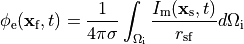
where are the potentials at a given field point,  ,
is the source density at a given source point,
,
is the source density at a given source point,  ,
and
,
and 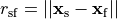 is the distance between source and field point.
A detailed description of the method and its limitation has been given in
(Bishop et al, IEEE Trans Biomed Eng 58(8), 2011),
is the distance between source and field point.
A detailed description of the method and its limitation has been given in
(Bishop et al, IEEE Trans Biomed Eng 58(8), 2011),
Bidomain simulations are the most appropriate approach when the heart is immersed in a volume conductor of limited size and the volume conductor can be represented. ECG recovery techniques are very well suited when the heart is immersed in an unbounded volume conductor. That is, ECG signals from a heart immersed in a torso can be approximated very well with a monodomain simulation using ECG recovery. On the other hand, ECG signals recorded at the surface of a Langendorff preparation are better approximated with a bidomain simulation when the heart is not immersed in a fluid bath. An alternative in this scenario is to use recovery method 3 where we use a monodomain simulation, but solve the elliptic PDE infrequently before outputting. Memorywise this simulation approach is equivalent to a bidomain simulations, in terms of execution speed the simulation is roughly equivalent to a monodomain simulation.
| field | type | description |
|---|---|---|
| phie_rec_ptf | string | file of recording sites (see Sref{sec:ptf} for format) |
| phie_recovery_file | Wfile | output file of ECG data |
| phie_rec_meth | Int | method to recover  |
A tutorial on how to use this ECG feature is found here.
Optical Mapping
To run an optical mapping experiment in post-processing,
both illuminating and emitting (or recording) surfaces need to be defined.
These are setup and defined like electrical electrodes being termed
illum_dbc and emission_dbc as they represent Dirichlet boundary conditions.
Like electrodes, they can be defined as a collection of points with boxes or with a list of vertices.
However, note that these points must lie on the surface of the tissue that you want to illuminate.
The illum_dbc.strength parameter should just be set to 1, although the magnitude does not really matter.
For now the em_dbc.strength is set to 0 on the surfaces from which you would like to compute the signal.
This is the most natural(ish) choice.
We assume that exactly just outside the tissue, there is no scattering, so photons zoom off to infinity,
thus leaving zero photon density just the other side of the boundary.
There is a more accurate mixed Neumann/Dirichlet boundary condition that could be implemented here,
but the differences are minimal (< 5 % between this and the more simple case of  .
In later versions, this other boundary condition may be added.
.
In later versions, this other boundary condition may be added.
| Variable | Type | Description | |
|---|---|---|---|
| num_illum_dbc | Int | Number of illumination Dirichlet boundary conditions | |
| num_emission_dbc | Int | Number of emmission Dirichlet boundary conditions | |
| optDT | Float | time step for optics in live mode,``0=no`` optics | |
| optics_mode | Int | Value | Description |
| 0 | Do not simulate optics | ||
| 1 | illuminate (for optogenetics simulations) | ||
| 2 | illumination and emission (optical maps) | ||
| phi_illum | Wfile | illumination photon source density,  |
|
| phi_em | Wfile | emission photon source density,  |
|
| w | Wfile | volumetric photon source density | |
| Vopt | Wfile | optical fluorescence signal | |
| mu_a_illum | Float | optical absorpitivity for illumination,  |
|
| Dopt_illum | Float | optical diffusitiviy for illumination,  |
|
| mu_a_em | Float | optical absorpitivity for emission,  |
|
| Dopt_em | Float | optical diffusitiviy for emission,  |
|
| illum_dbc | Optics_dbc* | boundary conditions for illumination | |
| emission_dbc | Optics_dbc* | boundary conditions for photon emission hline | |
Boundary Conditions
Like in the bidomain, on any surfaces which do not have a specific illumination or emission boundary condition imposed
we assume the standard zero flux condition of  .
This is ok for the sides of a slab, for example, which is being illuminated from its top side.
However, for the base of the slab this is not adequate,
and additional boundary conditions during both illumination and emission should be specified here.
Specifically,
.
This is ok for the sides of a slab, for example, which is being illuminated from its top side.
However, for the base of the slab this is not adequate,
and additional boundary conditions during both illumination and emission should be specified here.
Specifically,  should be defined on these surfaces.
This should only be worried about for thin slabs.
For anything thicker than
should be defined on these surfaces.
This should only be worried about for thin slabs.
For anything thicker than  or so, it does not really matter,
as the illuminating photon density will have decayed to almost zero here anyway
(although this should be adjusted for different illuminating wavelengths
which may penetrate deeper, as appropriate).
or so, it does not really matter,
as the illuminating photon density will have decayed to almost zero here anyway
(although this should be adjusted for different illuminating wavelengths
which may penetrate deeper, as appropriate).
| Variable | Type | Description |
|---|---|---|
| vtx_file | String | If specified, affected points given in this file |
| strength | Float | photon density on boundary |
| x0 | Float | lower z-ordinate of electrode volume |
| y0 | Float | lower y-ordinate of electrode volume |
| z0 | Float | lower z-ordinate of electrode volume |
| xd | Float | x-dimension of electrode volume |
| yd | Float | y-dimension of electrode volume |
| zd | Float | z-dimension of electrode volume |
| ctr_def | Flag | if set limits are [x0-xd x0+xd] etc, [x0 x0+xd] o.w. |
| geometry | Int | ID of dbc geometry definition |
| bctype | Short | 0=inomogeneous,1=homogeneous |
| dump_nodes | Flag | dump affected nodes in file |
Pre- and post-processing tools
In addition to using CARPentry directly for pre- and post-processing a number of specialized standalone tools is also available for specific purposes. The most widely used ones are summarized below.
Mesh generation (mesher)
Section author: Gernot Plank <gernot.plank@medunigraz.at>
Section author: Aurel Neic <aurel.neic@medunigraz.at>
Introduction
mesher is a program for generating simple regular FE meshes. It can also produce element tag regions
and fiber definitions during element generation.
Usage
The most important parameters of mesher are
- size : Set the size of the mesh in each axis direction.
- resolution : Set the resolution of the mesh in each axis direction.
- bath : Set the bath size in each axis direction. Negative sizes denote a bath on both sides.
- fibers : Set fiber rotation.
- mesh : Set output mesh name.
The unit of the size and resolution parameters is centimeters, while the unit of the resolution is set in micrometers.
Fiber orientation is assigned based on following assumptions:
- The negative z axis is the transmural direction.
- The positive y axis is the apico-basal direction.
- The positive x axis is the circumferential direction.
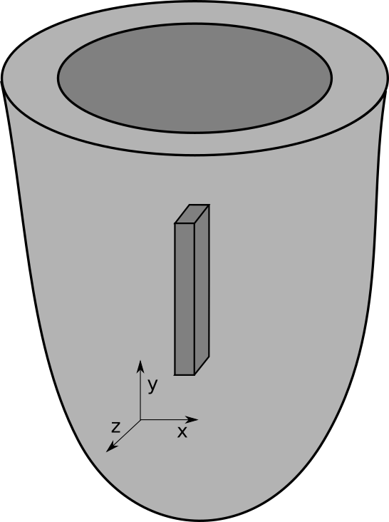
Convention for the wedge orientation.
Example
The following example creates a myocardial slab of dimensions 0.05 x 0.6 x 0.3 cm immersed in a bath of 0.02 cm on each side:
$ bin/mesher \\
-size[0] 0.05 \\
-size[1] 0.6 \\
-size[2] 0.3 \\
-bath[0] -0.02 \\
-bath[1] -0.02 \\
-bath[2] -0.02 \\
-resolution[0] 100.0 \\
-resolution[1] 100.0 \\
-resolution[2] 100.0 \\
-mesh block
By default, the geometry’s center is located at (0,0,0). As specified, the bounding box of the intracellular domain is
Bbox:
x: (      -250.00 ,       250.00 ), delta 500.00
y: (     -3000.00 ,      3000.00 ), delta 6000.00
z: (     -1500.00 ,      1500.00 ), delta 3000.00
while the bounding box of the overall mesh is
Bbox:
x: (      -450.00 ,       450.00 ), delta 900.00
y: (     -3200.00 ,      3200.00 ), delta 6400.00
z: (     -1700.00 ,      1700.00 ), delta 3400.00
Rule-based fibers can be added with the parameters in the fibers parameter structure. In the previous
example, fiber rotation can be added with:
-fibers.rotEndo 60 \\
-fibers.rotEpi -60 \\
-fibers.sheetEndo 90 \\
-fibers.sheetEpi  90 \\
The resulting geometry is:
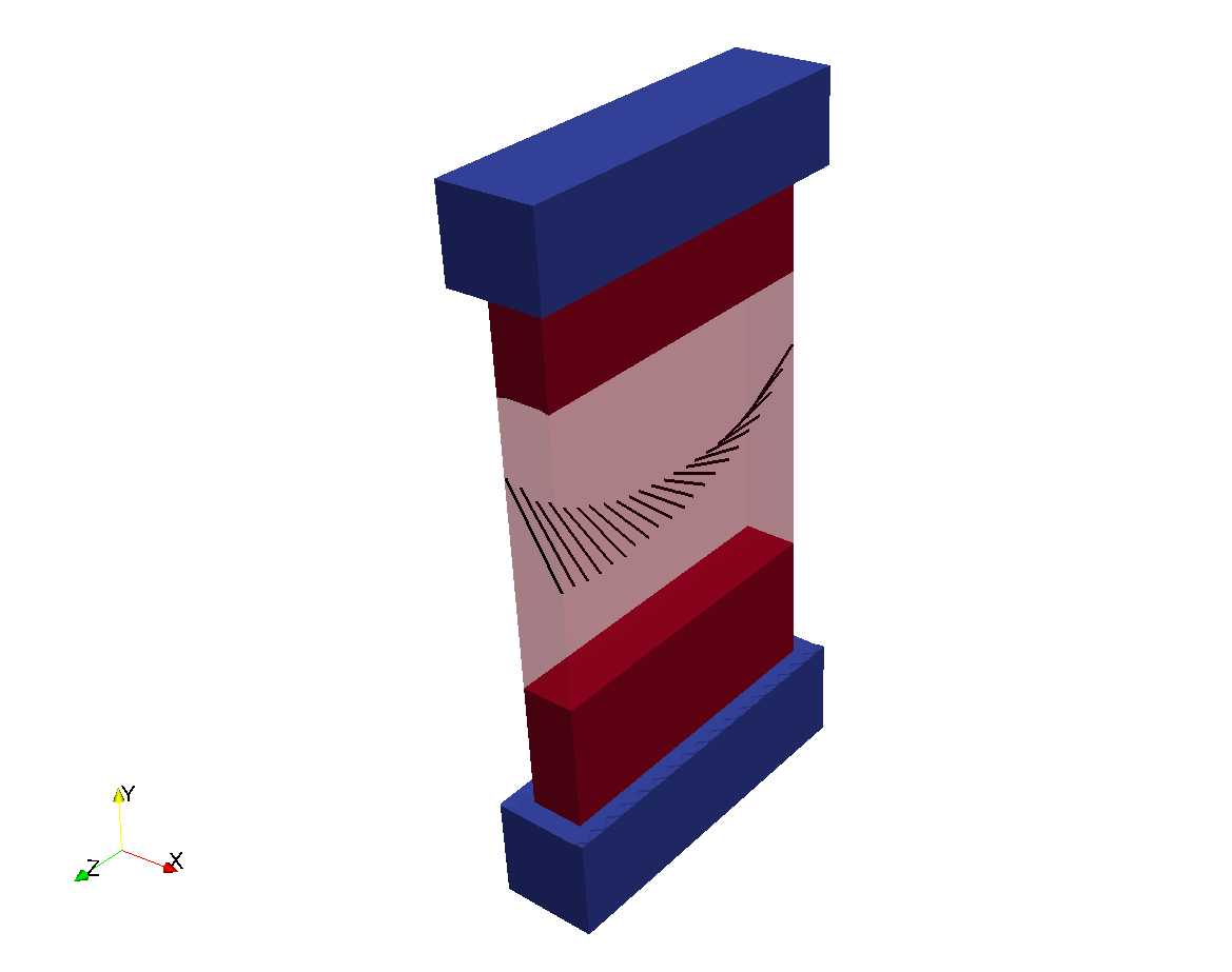
A slab mesh produced by mesher.
Tag regions
By default, element tag region 0 is assigned to the bath and region 1 is assigned to the myocardium.
Additional regions can be assigned via regdef parameters. A regdef parameter defines a geometric
shape. Elements inside this shape are assigned a given element tag.
The supported region definition shapes are:
$ mesher +Help regdef[0].type

regdef[0].type:
    how to define region

    type:   Int
    default:(Int)(0)
    menu: {
            (Int)(2)        cylinder
            (Int)(1)        sphere
            (Int)(0)        block
    }
The following example shows a minimal definition of a block region:
-numRegions      1 \\
-regdeg[0].type  0 \\
-regdef[0].tag   TAG \\
-regdef[0].p0[0] P0X \\
-regdef[0].p0[1] P0Y \\
-regdef[0].p0[2] P0Z \\
-regdef[0].p1[0] P1X \\
-regdef[0].p1[1] P1Y \\
-regdef[0].p1[2] P1Z \\
Mesh processing (meshtool)
Section author: Aurel Neic <aurel.neic@medunigraz.at>
Mesh data extraction
Submesh extraction
With the “extract mesh” mode, a submesh can be extracted from a mesh based on tag regions. The mode’s parameters are as following:
$ meshtool extract mesh

Mesh extract error: Insufficient parameters provided.
extract mesh: a submesh is extracted from a given mesh based on given element tags
parameters:
-msh=<path>         ... (input) path to basename of the mesh to extract from
-tags=tag1,tag2     ... (input) ","-seperated list of tags
-ifmt=<format>      ... (optional) mesh input format. may be: carp_txt, carp_bin, vtk, vtk_bin, mmg, stellar
-ofmt=<format>      ... (optional) mesh output format. may be: carp_txt, carp_bin, vtk, vtk_bin, vtk_polydata, mmg, stellar
-submsh=<path>      ... (output) path to basename of the submesh to extract to
Therefore a typical call would be:
meshtool extract mesh -msh=/home/aneic/meshes/TBunnyC/mesh/TBunnyC -submsh=TBC_125 -tags=125
Both input and output mesh formats are the default CARP-text formats. In addition to the submesh, meshtool also writes two *.nod and *.eidx files. These hold the node and element mappings between the submesh and the original mesh and are needed by modes that relate submeshes with their associated meshes (e.g. the “insert” and “map” modes).
Surface extraction
Meshtool offers a potent interface for mesh surface extraction. The mode’s help description is:
$ meshtool extract surface

Surface extract error: Insufficient parameters provided.
extract surface: extract a sequence of surfaces defined by set operations on element tags
parameters:
-msh=<path>           ... (input) path to basename of the mesh
-surf=<path>          ... (output) list of names associated to the given operations
-op=operations        ... (optional) list of operations to perform. By default, the surface of the full mesh is computed.
-ifmt=<format>        ... (optional) mesh input format. may be: carp_txt, carp_bin, vtk, vtk_bin, mmg, purk, stellar
-ofmt=<format>        ... (optional) mesh output format. may be: carp_txt, carp_bin, vtk, vtk_bin, vtk_polydata, mmg, stellar
-edge=<deg. angle>    ... (optional) surface elements connected to sharp edges will be removed. A sharp edge is defined
                          by the nodes which connect elements with normal vectors at angles above the given threshold.
-coord=<xyz>:<xyz>:.. ... (optional) restrict surfaces to those elements reachable by surface edge-traversal
                          from the surface vertices closest to the given coordinates.
                          If -edge= is also provided, sharp edges will block traversal, thus limit what is reachable.
-size=<float>         ... (optional) surface edge-traversal is limited to the given radius from the initial index.

The format of the operations is:
tagA1,tagA2,..[+-:]tagB1,tagB2../tagA1,..[+-:]tagB1../..
Tag regions separated by "," will be unified into submeshes. If two submeshes are separated by "-", the rhs mesh surface
will be removed from the lhs surface (set difference). Similarly, using "+" will compute the surface union.
If the submeshes are separated by ":", the set intersection of the two submesh surfaces will be computed.
Individual operations are separated by "/".
The number of names provided with "-surf=" must match the number of operations. If no operations are provided,
the surface of the whole geometry will be extracted. Individual names are separated by ",".
Further restrictions can be added to the surface extraction with the -edge= , -coord= , -size= options.
The surface of a whole mesh can therefore be extracted with:
$ meshtool extract surface -msh=TBC_i -surf=TBC_i
Reading mesh: TBC_i.*
Reading elements in text CARP format:                       [====================]
Reading points in text CARP format:                         [====================]
Reading fibers (2 directions) in text CARP format:          [====================]
Done in 7.47963 sec
Computing surface 1/1
Done in 0.870943 sec
Writing surface TBC_i.surf
Writing vertices TBC_i.surf.vtx
Writing neubc TBC_i.neubc
Done in 0.103977 sec
Here, a surface TBC_i.surf is generated for the mesh TBC_i.elem, TBC_i.pts. Further, *.surf.vtx file (holding the unique surface vertices) and a *.neubc file (containing data needed for mechanics Neumann boundary conditions) are written. If “-ofmt” is specified, the surface is also outputted as a standalone mesh in the desired format.
More complex surfaces can be extracted with set operations on tag sets. For this, the “-op” parameter needs to be specified. In the following example, the set intersection of the surface of tag region 125 and the surface of tag region 150 is computed:
meshtool extract surface -msh=TBC_i -surf=TBC_i_125:150 -op=125:150
The result looks like:
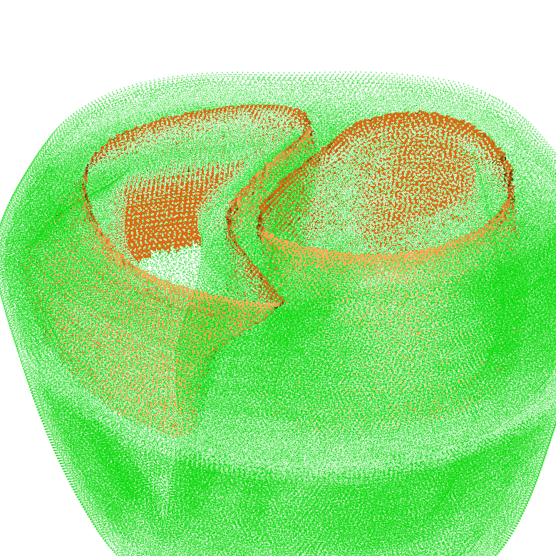
The surface intersection between tags 125 and 150.
Finally, surfaces can be computed by traversing the surface nodes connected to a given node list. Sharp edges can be set to block surface traversal. The “-edge” parameter defines the sharp edge angle threshold between surface elements. For example the base of the TBunnyC myocardium can be computed as following:
$ meshtool extract surface -msh=TBC_i -surf=TBC_i.top -idx=506478 -edge=10
Reading mesh: TBC_i.*
Reading elements in text CARP format:                       [====================]
Reading points in text CARP format:                         [====================]
Reading fibers (2 directions) in text CARP format:          [====================]
Done in 7.49793 sec
Setting up n2e / n2n graphs ..
Computing connectivity graphs:                              [====================]
Computing surface 1/1
Done in 0.859898 sec
Computing connectivity graphs:                              [====================]
Nodes reached:                                              [====================]
Writing surface TBC_i.top.surf
Writing vertices TBC_i.top.surf.vtx
Writing neubc TBC_i.top.neubc
Done in 0.460613 sec
The result looks like:
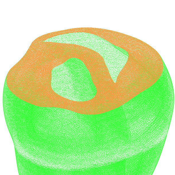
The surface of the TBunnyC myocardium base.
Meshtool query function
Query list of tags
meshtool query tags -msh=MESHNAMEWITHOUTEXTENSION -ifmt=%
where % is either carp_txt, carp_bin, vtk, vtk_bin depending on the mesh to be checked. In case you are checking a vtk file make sure that the name of the tag variable in the vtk file is “elemTag”. This command prints a list of all tags comprised in the mesh. An example output is shown below:
Reading mesh: /home/plank/meshes/TBunnyC2/mesh/TBunnyC2.*
Reading elements in text CARP format:                       [====================]
Reading points in text CARP format:                         [====================]
Reading fibers (2 directions) in text CARP format:          [====================]
Done in 0.638392 sec
All tags:
0 1 2 100 101 102 103 104 105 106 150 151 152 153 154 155 156 200 201 202 203 204 205 206
Extracting myocardium ..
Done in 0.220971 sec
Myocardium tags:
100 101 102 103 104 105 106 150 151 152 153 154 155 156 200 201 202 203 204 205 206
Retrieve resolution statistics of a mesh
Mean and variability of edge lengths in a FEM mesh is an important metric as spatial resolution influences to some degree numerical computation. An edge lengths statistics is retrieved by
meshtool query edges -msh=MESHNAMEWITHOUTEXTENSION -ifmt=%
This plots a text-based edge length histograms to the console:
Reading mesh: /home/plank/meshes/TBunnyC/mesh/TBunnyC.*
Reading elements in binary CARP format:                     [====================]
Reading points in binary CARP format:                       [====================]
Done in 2.92863 sec
Setting up n2e / n2n graphs ..
Computing connectivity graphs:                              [====================]
Done in 3.47954 sec

Number of connections

Average: 13.8348, (min: 4, max: 31)

 == Histogramm ==

         --------------------------------------------------------------------------------------------
   +0.26 |                                   *                                                      |
         |                               *****                                                      |
   +0.22 |                             **     *                                                     |
         |                           **       *                                                     |
         |                       ****         **                                                    |
         |                     ***             *                                                    |
   +0.15 |                     *               *                                                    |
         |                    **                *                                                   |
         |                    *                 *                                                   |
         |                   **                 **                                                  |
   +0.07 |                   *                   *                                                  |
         |                  **                   *                                                  |
         |                  *                    ***                                                |
         |               ****                      *****                                            |
   +0.00 |****************                             ****************************************     |
         --------------------------------------------------------------------------------------------
          4.0             8.9            13.7            18.6            23.4            28.3

Edge lengths

Average: 326.493, (min: 37.0675, max: 1840.16)

 == Histogramm ==

         --------------------------------------------------------------------------------------------
   +0.53 |                                                                                          |
         |        **                                                                                |
   +0.46 |        ***                                                                               |
         |       ** *                                                                               |
         |       *  **                                                                              |
         |       *   **                                                                             |
   +0.30 |      **    *                                                                             |
         |      *     **                                                                            |
         |      *      **                                                                           |
         |     **       *                                                                           |
   +0.15 |     *         *                                                                          |
         |     *         **                                                                         |
         |    *           **                                                                        |
         |  ***            ****                                                                     |
   +0.00 |***                 *****************************************************************     |
         --------------------------------------------------------------------------------------------
         37.1           361.2           685.4          1009.5          1333.7          1657.8
Retrieve mesh quality statistics
A statistics on mesh quality can also be retrieved using the query command. So far, quality calculation is only implemented for tetrahedral elements. In tissue scale simulations it is a frequent source of errors that meshes are generated without properly checking element quality.
meshtool query quality -msh=MESHNAMEWITHOUTEXTENSION -ifmt=%
Shown below is a mesh quality histogram as output to the console. The quality metric outputs the quality of an element on a scale ranging from 0 to 1 where 0 indicates best quality and 1 is poorest quality.
Reading mesh: /home/plank/meshes/TBunnyC/mesh/TBunnyC.*
Reading elements in binary CARP format:                     [====================]
Reading points in binary CARP format:                       [====================]
Done in 0.491191 sec
Computing mesh quality ..
Done in 0.202803 sec

-------- mesh statistics ---------
Number of elements: 5082272
Number of nodes: 862515

-------- element quality statistics ---------
Used method: tet_qmetric_weightedShapeDist with 0 == best, 1 == worst
Min: 3.98307e-05 Max: 0.873355 Avrg: 0.125359

Histogramm of element quality:

         --------------------------------------------------------------------------------------------
   +0.12 |                                                                                          |
   +0.12 |      ****                                                                                |
         |     **  **                                                                               |
         |    **    **                                                                              |
         |    *      *                                                                              |
   +0.09 |   **      **                                                                             |
         |   *        *                                                                             |
         |  **        **                                                                            |
         |  *          *                                                                            |
   +0.07 | **          **                                                                           |
         | *            *                                                                           |
         | *            **                                                                          |
         | *             *                                                                          |
   +0.05 |*              **                                                                         |
         |*               **                                                                        |
         |*                *                                                                        |
         |*                **                                                                       |
   +0.02 |                   **                                                                     |
         |                    **                                                                    |
         |                     ***                                                                  |
         |                       *****                                                              |
   +0.00 |                           ************************************************************** |
         --------------------------------------------------------------------------------------------
          0.0             0.2             0.4             0.5             0.7             0.9
Mesh quality improvement
In the “clean quality” mode, the quality of a mesh can be improved by vertex displacement and by volumetric smoothing. The effectiveness of either methods depends on the reason for the bad element quality (e.g. mesh has been clipped, mesh has been smoothed).
Vertex displacement restores quality for elements that have been “flattened-out”, either explicitly by mesh smoothing, or implicitly by the mesh generation algorithm. It’s drawback is that it destroys surface smoothness.
Vertex smoothing redistributes vertices in equal distance of each other. This improves mesh quality if the mesh has been modified by clipping.
The two methods can be used alone or combined. Depending on the underlying mesh problem, they can complement or act against each other. For example, if the mesh generation algorithm was configured to produce very smooth surfaces, it has probably also produced flat elements at the interfaces of the surfaces. This flat elements can only by improved by vertex displacement which will reduce surface smoothness. Vertex smoothing is not useful for this case, since it would only counter the vertex displacement by restoring surface smoothness.
In the following example, the mesh quality is restored for a LV mesh where an artery has been clipped. Here, mesh smoothing will be generate the main quality improvement. Therefore, the smoothing coefficient (smth=0.3 means that a vertex will be moved 30 percent towards its center-point) and number of iterations (iter=150) are set rather high. Surface files are passed via the “surf” parameter, in order to protect them and their edges (edge detection is turned on via edge=30).
$ meshtool clean quality -msh=OPBG010.cut -thr=0.9 -surf=OPBG010.cut,OPBG010.cut.blood -smth=0.3 -iter=150 -edge=30 -outmsh=OPBG010.cut.cln -ofmt=vtk_bin
Using OpenMP parallelization with 6 threads.
Reading mesh: OPBG010.cut.*
Reading elements in text CARP format:                       [====================]
Reading points in text CARP format:                         [====================]
Reading fibers (1 direction) in text CARP format:           [====================]
Mesh consists of 2191988 elements, 383188 nodes.
Correcting inside-out tets ..
Pass 1: Corrected 0 inside-out elements.
Done in 3.48826 sec
Reading surface: OPBG010.cut.surf
Reading elements in text CARP format:                       [====================]
Reading surface: OPBG010.cut.blood.surf
Reading elements in text CARP format:                       [====================]
Setting up n2e / n2n graphs for mesh surface ..
Computing connectivity graphs:                              [====================]
Setting up line interfaces for mesh surface ..
Computing connectivity graphs:                              [====================]
Computing connectivity graphs:                              [====================]
Done in 5.89264 sec

Checking mesh quality ..
Mesh quality statistics:
min: 6.69769e-05, max: 2.78184, avg: nan
Number of elements above threshold: 1381
Done in 0.15244 sec

Improving mesh ..
Setting up n2e / n2n graphs for mesh ..
Computing connectivity graphs:                              [====================]
Starting with optimization ..
Iter 0: Number of elements left above threshold: 1381
Smoothing progress:                                         [====================]
Smoothing progress:                                         [====================]
Smoothing progress:                                         [====================]
Smoothing progress:                                         [====================]
Iter 1: Number of elements left above threshold: 51
Smoothing progress:                                         [====================]
Smoothing progress:                                         [====================]
Smoothing progress:                                         [====================]
Smoothing progress:                                         [====================]
Iter 2: Number of elements left above threshold: 64
Mesh quality statistics:
min: 6.69769e-05, max: 0.997674, avg: 0.105546
Done in 12.1368 sec
Correcting inside-out tets ..
Pass 1: Corrected 20 inside-out elements.
Pass 2: Corrected 0 inside-out elements.
Writing mesh: OPBG010.cut.cln.*
Writing vtk file in binary format:                          [====================]
Done in 1.15729 sec
The original mesh had element of such a poor quality that the element quality couldn’t even be computed, while the resulting mesh is of useable quality.
The result looks like:
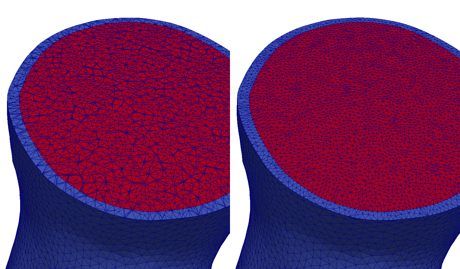
Comparison between original mesh and imporved mesh for a clipped geometry.
igbutils
For all tools, help is output with the -h option.
igbhead
Operations to perform on the headers of IGB files. Most commonly, it it used to print the header information but can also be usd to modify it. This utility can also be used to change the storage type of the file, or put an IGB header on to ASCII and binary data file.
igbapd
A simple utility to compute action potential durations.
igbops
This utility can perform basic math operations on one or two IGB files. There are preset functions as well as a parser for arbitrary functions. For example, one can difference two IGB files, find maxima over time, or apply a box filter.
igbextract
This is a tool to extract a hyperslab of data from an IGB file. The format of the output can be chosen between ASCII, binary or IGB.
igbdft
This is a tool for simple frequency domain techniques. It contains a limited number of operations which include Butterworth filtering, DFTs, and computing phase.
FEM tools
Tools recognize the -h to display detailed help.
GlElemCenters
Compute the element centers of a nodally defined mesh
GlFilament
Compute phase singularities and filaments.
GlGradient
Compute gradients of grid data and conduction velocities if activation times are used.
GlInterpolate
Interpolate data restitution-protocol-definition, from nodes to element centers or vice versa.
GlRuleFibers
Compute the fibres for a biventricular mesh
GlTransfer
Transfer data between spatially overlapping grids
Visualization tools
Meshalyzer
Purpose
Meshalyzer is a program for displaying unstructured grids, visualizing data on the grid, as well as examining the structure of the grid. It is an ever changing and ongoing project that has been in development since 2001.
Installation
Meshalyzer uses the Fast Light Tool Kit (“FLTK”) to provide modern GUI functionality. It supports 3D graphics via OpenGL TM and its build-in GLUT emulation. Before getting the software from a GitHub repository, a version 1.3.x of FLTK needs to be provided on your system by either installing it through the package manager or compiling it from the sources:
cd <installation-directory>
wget http://fltk.org/pub/fltk/1.3.4/fltk-1.3.4-1-source.tar.gz
tar -xzvf fltk-1.3.4-1-source.tar.gz
cd fltk-1.3.4-1
./configure --enable-xft --enable-shared
make
sudo make install
cd ..
Note
FLTK has some additional dependencies in order to be successfully compiled. A list of typically missing packages is given here. Be aware that the package names could slightly deviate across common operating systems.
- libpng-dev
- libjpeg-turbo-dev
- freeglut3-dev
- libXft-devel
- [ libpthread-stubs0-dev ]
Hence, get Meshalyzer from the freely available GitHub repository and finish your installation.
cd <installation-directory>
git clone https://github.com/cardiosolv/meshalyzer
cd meshalyzer
make
Input Files
Meshalyzer assumes that there is a model, defined by a set of vertices, which is to be displayed. Beyond that, everything is optional. The vertices may be connected to form structures, specifically cables, triangular elements, quadrilaterals, tetrahedra, hexahedra, prisms, or simple line segments. Scalar data may be associated with every point on the grid and may be used to colour any of the connected structures. An auxiliary set of points may also be defined on which to display vector data,
Furthermore, the points may be divided into different regions which may have their attributes independently manipulated. Regions are delimited by tagged volume elements (see Sref{sec:voleles}), or may be specified by a range of vertices (see~Sref{sec:regfile}), As well, all the structures formed by those vertices are part of the region. Vertices may belong to more than one region, and there is at least one region in a grid. If a region is not specified, all structures belong to the default region. If there is a element direction file (.lon file), and no volume elements are tagged, elements with no direction will be region 0, and other elements will be region 1.
Surfaces may be formed from collections of two-dimensional elements.
Surfaces are defined by surface element files (see Sref{sec:surffile}).
Also, surfaces are defined if there are any 2D elements in an elem
file (see Sref{sec:elem}).
In the latter case,
the 2D elements are placed in different surfaces based on their region number.
Surfaces are independent of regions, and the relationship between the points
and model structures is described in the fig-UML.
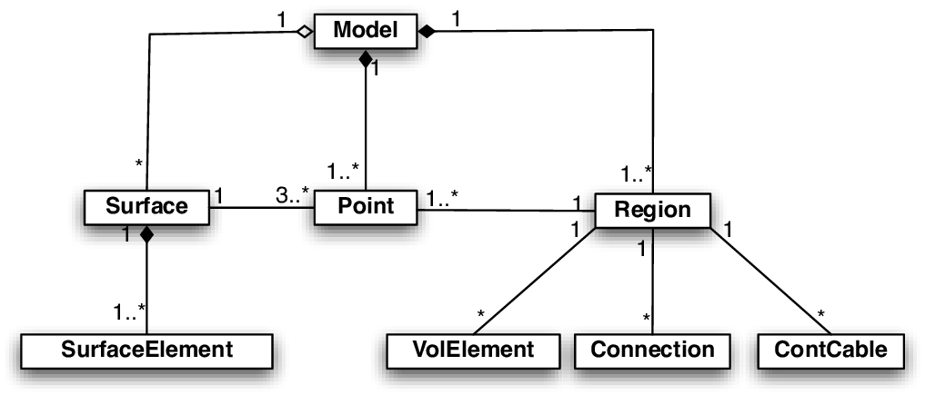
Relationship between vertices (Points) and other structures.}
All files (except IGB files) are ASCII files.
They may be gzipped in which case .gz should be appended to the extensions given below.
Note that files are scanned line by line
and that extra information on each line is ignored by meshalyzer.
Vertices
The file defining vertices in the model is the only mandatory file.
It must have the extension .pts following the carpentry format for nodal files.
The base name of this file, i.e., without the extension, is
used as the base name for cables, connections, triangles,
tetrahedra files, and shells files.
Appendix
File formats
Input file formats
When setting up a CARP simulation, a node, element and fibre files will generally be required. They must be given the same base name, but different extensions, for example:
meshname.pts
meshname.elem
meshname.lon
To support the quick variation of fiber architecture alternative fiber files can be provided using the orthoname option. In this case meshname is used for nodal and element file, but orthoname is used for the fiber file. For instance, using
-meshname biv_rabbit -orthoname biv_rabbit_hf
would read the following files:
biv_rabbit.pts
biv_rabbit.elem
biv_rabbit_hf.lon
Node file
Extension: .pts
The node (or points) file starts with a single header line with the number of nodes,
followed by the coordinate of the nodes, one per line, in  .
For example, for a mesh with nodes we have:
.
For example, for a mesh with nodes we have:
| Format | Example |
|---|---|
|
10000 |
 |
10.3400 -15.0023 12.023 |
 |
11.4608 -12.0237 11.982 |
 |
|
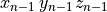 |
-8.4523 36.7472 4.6742 |
Element File
Extension: .elem
In general, CARPentry supports various types of elements which can be mixed in a single mesh. However, not all element types are supported in every context, some limitations apply. In electrophysiology simulations element types can be mixed, whereas in mechanics only tetrahedral and hexahedral elements are support. The simple native element file format is as follow
The file begins with a single header line containing the number of elements, followed by one element definition per line. The element definitions are composed by an element type specifier string, the nodes for that element, then optionally an integer specifying the region to which the element belongs.
For example, for a mesh with elements and where
 is the type specifier of element ,
 indices the
  -th node of element ,
 is the number of nodes of element and
 is the optional region of element ,
the format is given as:
| Format | Example |
|---|---|
|
20000 |
![T_0 \, N_{0,0} \, N_{0,1} \ldots N_{0,m_i-1} \, [r_0]](_images/math/ad98e8d53e30f7e20f26741a71868844706c94af.png) |
Tt 10 15 123 45 1 |
![T_1 \, N_{1,0} \, N_{1,1} \ldots N_{1,m_i-1} \, [r_1]](_images/math/23595fd5bda2322e1bc352655d76404416808584.png) |
Pr 45 36 100 54 35 74 0 |
|
|
![T_{n-1} \, N_{n-1,0} \, N_{n-1,1} \ldots N_{n-1,m_i-1} \, [r_{n-1}]](_images/math/131d78db40ddae8bd3ed8e030c25933f81303dfe.png) |
Tt 9374 7432 1234 4532 1 |
The node indicies are determined by their order in the points file. Note that the nodes are 0-indexed, as indicated in Sec. Node file above. The element formats supported in CARP, including their element type specifier strings are given in table Element types supported in CARPentry for different physics. Electrophysiology (EP), Mechanics (MECH) and Fluid (FL). *: for internal use only, not supported in mesh files.. The ordering of nodes in each of the 3D element types is shown in Nodal ordering of 3D element types.
| Type Specifier | Description | Interpolation | #Nodes | Supported in |
|---|---|---|---|---|
| Ln | Line | linear | 2 | EP |
| cH * | Line | cubic | 2 | HPS |
| Tr | Triangle | linear | 3 | EP |
| Qd | Quadrilateral | Ansatz | 4 | EP |
| Tt | Tetrahedron | linear | 4 | EP, MECH, FL |
| Py | Pyramid | Ansatz | 5 | EP |
| Pr | Prism | Ansatz | 6 | EP |
| Hx | Hexahedron | Ansatz | 8 | EP |
Nodal ordering of 3D element types
Fiber file
Extension: .lon
Fibres are defined in CARP on a per-element basis. They may be defined by just the fibre direction, in which case a traversely isotropic conductivity or mechanics material model must be used, or additionally specifying the sheet (or transverse) direction to allow full orthotropy in the model.
The file format starts with a single header line with the number of fibre vectors defined in the file (1 for fibre direction only, 2 for fibre and sheet directions), and then one line per element with the values of the fibre vector(s). Note that the number of fibres must equal the number of elements read from the element file.
For example, where  is the number of fibre vectors (1 or 2),
 are the components of the fibre vector for element and
 are the components of the sheet vector for element :
| Format | Example |
|---|---|
|
2 |
![f_{0,x} \, f_{0,y} f_{0,z} \, [s_{0,x} \, s_{0,y} s_{0,z}]](_images/math/e235747f8fe95364d6fdef8587330baab98027f1.png) |
0.831 0.549 0.077 0.473 -0.775 0.417 |
![f_{1,x} \, f_{1,y} f_{1,z} \, [s_{1,x} \, s_{1,y} s_{1,z}]](_images/math/1d795785895d8ed68ac4fff2b2cde420a01527a3.png) |
0.647 0.026 0.761 -0.678 0.475 0.560 |
|
|
![f_{n-1,x} \, f_{n-1,y} \, f_{n-1,z} \, [s_{n-1,x} \, s_{n-1,y} \, s_{n-1,z}]](_images/math/ce1dda8534323b874499f9931a8967ec2be229f7.png) |
0.552 0.193 0.810 -0.806 0.369 0.462 |
The fibre and sheet vectors should be orthogonal and of unit length.
Vertex file
Extension: .vtx
An collection of preferably unique mesh indices may be stored in a vertex file.
| Format | Example |
|---|---|
| N # number of nodes | 192 |
| intra|extra # definition domain | intra |
| node_0 | 47 |
| node_1 | 123 |
|
|
| node_N-1 | 23943 |
Note
- A stimulus electrode file, e.g. apex.vtx may be added in the parameter file as follows:
-stimulus[0].vtx_file apex
The extra-domain refers to the entire user-specified mesh.
The intra-domain refers to the geometry where non-zero fibers were defined.
Although intra and extra should be the the same for tissue-only geometries, CARPentry/mechanics may not like vtx-files stating the vertices as intra domain.
Purkinje file
Extension: .pkje
The format of the Purkinje file is very specific and must be followed carefully.
The # character begins a comment. It and everything following on a line are ignored.
Section purk-file-rules gives the exact rules for defining Purkinje networks.
Below there are comments explaining the different fields inside the file Purkinje.pkje.
Number_of_Cables
Cable 0
Father1 Father2
Son1 Son2
Nodes_Cable
Size
Gap_junction_resistance
Intracellular_conductivity
Node1_x Node1_y Node1_z
...
NodeN_x NodeN_y NodeN_z
Cable 1
...
Note that if a parent or son is unassigned, it is Father2 or Son2 that is assigned a value of -1. An example of a few lines from a Purkinje file follows:
97      # Number of Cables present in the tree [0-96]
Cable 0 # Cable 0 is always the first
-1 -1   # no Fathers for Cable 0
1 2     # Son 1 and Son 2
4       # Number of nodes in this Cable
75      # Relative size of cable (i.e. #parallel fibres or cross-sectional area)
100.0   # gap junction resistance (kOhm)
0.0006  # conductivity (Ohm-cm)
1100 -3400 2200 # NODE 1
1149 -3300 2178 # NODE 2
1184 -3201 2165 # NODE 3
1201 -3090 2154 # NODE 4
Cable 1 # Cable 1, (order must be followed)
0 -1    # FATHER1 = Cable 0, no Father2
3 -1    # SON1 = Cable 3, no Son2
80      # Number of nodes = 80
7.0
100.0
0.0006
1201 -3090 2154
1245 -3020 2143
1209 -2975 2133
.
.
.
Hint
missing link target purk-file-rules
Purkinje-myocardial junction (PMJ) tuning file
After the global PMJ parameters are applied, individual junction parameters are set based on values in a file. Cables specified must have a PMJ.
#junctions
cable_no R_PMJ PMJ_scale
cable_no R_PMJ PMJ_scale
    .
    .
    .
cable_no R_PMJ PMJ_scale
Pulse file
Note that time values must increase, that is,

N # Number_of_samples
t0  val0
t1  val1
.
.
.
t(N-1)  val(N-1)
Vertex adjustment file
N           # Number_of_nodes
intra|extra # definition domain
node_0 val_0
node_1 val_1
.
.
.
node_n-1 val_n-1
Neumann boundary file
Restitution protocol definition file
To be completed Output file formats ——————-
IGB files
Extension: .igb
CARP simulations usually export data to a binary format called IGB.
IGB is a format developed at the University of Montreal
and originally used for visualizing regularly spaced data.
An IGB file is composed of a 1024-byte long header followed by binary data
which is terminated by the ASCII form feed character (^L / character 12).
For unstructured grids, the individual dimensions are meaningless
but x  y`
y` z should be equal to the number of vertices.
The header is composed of strings of the following format,
separated by white space: KeyWord:value
Note that the header must be padded to 1024 bytes.
The first block of key words in IGB keywords need to be specified. The rest are optional.
| KeyWord | Type | Description |
|---|---|---|
| x | int | number of samples in x |
| y | int | number of samples in y |
| z | int | number of samples in z |
| t | int | number of samples in t |
| systeme | string | big_endian or little_endian |
| type | string | binary data type: byte, char, short, long, float, double, int, uint, vec3f, vec4f, vec3d, vec4d |
| unites | string | units of data |
| facteur | float | scaling factor for data |
| zero | float |
|
| org_x | float | lower right x coordinate |
| org_y | float | lower right y coordinate |
| org_z | float | lower right z coordinate |
| org_t | float | time of first slice |
| inc_x | float | distance between x samples |
| inc_y | float | distance between y samples |
| inc_z | float | distance between z samples |
| inc_t | float | time between samples |
| dim_x | float | extent in x |
| dim_y | float | extent in y |
| dim_z | float | extent in z |
| dim_t | float | duration |
| unites_x | string | units of measure for spatial x dimension |
| unites_y | string | units of measure for spatial y dimension |
| unites_z | string | units of measure for spatial z dimension |
| unites_t | string | units of measure for time |
| comment | string | arbitrary comment |
| aut_name | string | author’s name |
| transparent | hex | value for no data |
Dynamic Points
Extension: .dynpts
Points may also move in space as functions of time. This is often associated with displacement during contraction, for example. The number of points must remain constant for all time instances, as well as the elements defined by them. Dynamic point files use the IGB format (see IGB files) with data type vec3f.
Vector data files
Extension: .vec and .vpts
To display vector data, an auxiliary set of points must be defined by a file with the .vpts suffix. It follows the same format as the Node file. A file with the same base name but having the extension .vec defines the vector and scalar data. It has the following format:
| Format |
|---|
data.x data.y data.z [scalar_datum] |
data.x data.y data.z [scalar_datum] |
|
data.x data.y data.z [scalar_datum] |
The scalar datum, as indicated, is optional. The .vec format can also be used
for visualization of fiber orientations stored in .lon files.
For this sake, a .vpts file must be generated
holding the coordinates of the centers of each element in the mesh.
This is conveniently achieved with GlElemCenters
and changing the fiber file extension to .vec.
For example, for a mesh with elements
and where  corresponds to the components of the fiber vector :
| Format | Example |
|---|---|
 |
8.12453e-01 -2.22623e-01 1.25001e00 |
 |
5.68533e-01 -1.81807e-01 1.04956e00 |
|
|
 |
5.70671e-01 -1.67572e-01 1.06615e00 |
Vector data can also be input as an IGB file using the types vec3f, vec4f, vec3d, vec4d where 3 or 4 refers to the number of elements in each datum, and d and f refer to float or double. The first 3 elements define the value of the vector field, and the optional 4-th element is the scalar component as above. This file has the suffix .vec.igb.
Auxiliary Grid
Extensions: .pts_t, .elem_t, .dat_t
This format is used by Introduction to meshalyzer to display additional data on an auxiliary grid. The grid may contain any of the elements forming the main grid (points,lines,surface elements,volume elements), and the elements may change as a function of time. If scalar data has already been read in, the number of time instances in the auxiliary grid must either be one, or the same as the scalar data. The points file may have only one time instance, which is then assumed constant over all time.
A vertex file is mandatory and has the extension .pts_t. An element file is optional. If present, it has the same base name as the vertex file but with the extension .elem_t. Scalar data may also be optionally defined on the auxiliary grid. The file has the same basename as the vertex file but with the extension .dat_t. The file formats follow:
| .pts_t | .elem_t | .dat_t | ||
|---|---|---|---|---|
| #times | #times | #times | ||
| #points_time0 | #elements_time0 | #data_time0 | ||
| pt(0,0).x | pt(0,0).y | pt(0,0).z | element(0,0) | data(0,0) |
| pt(1,0).x | pt(1,0).y | pt(1,0).z | element(1,0) | data(1,0) |
| . | . | . | . | . |
| . | . | . | . | . |
| . | . | . | . | . |
| . | . | . | element(M,0) | . |
| . | . | . | #elements_time1 | . |
| . | . | . | element(0,1) | . |
| . | . | . | element(1,1) | . |
| . | . | . | . | . |
| pt(N,0).x | pt(N,0).y | pt(N,0).z | . | data(N,0) |
| #points_time1 | . | #data_time1 | ||
| pt(0,1).x | pt(0,1).y | pt(0,1).z | . | data(0,1) |
| pt(1,1).x | pt(1,1).y | pt(1,1).z | . | data(1,1) |
| . | . | . | . | . |
| . | . | . | element(M,1) | . |
| . | . | . | #elements_time2 | . |
| . | . | . | element(0,2) | . |
| . | . | . | . | . |
CARPentry Literature
The methodological underpinnings of virtually all features and concepts implemented in CARPentry were reported in detail in various journal publications. A selected non-exhaustive list of papers is found below.
| [1] | Bayer JD1, Blake RC, Plank G, Trayanova NA.
A Novel Rule-Based Algorithm for Assigning Myocardial Fiber Orientation to Computational Heart Models,
Ann Biomed Eng 40(10):2243-54, 2012. [PubMed]
[pdf] |
| [2] | Plank G, Liebmann M, Weber dos Santos R, Vigmond EJ, Haase G.
Algebraic multigrid preconditioner for the cardiac bidomain model,
IEEE Trans Biomed Eng. 54(4):585-96, 2007.
[PubMed]
[pdf]. |
| [3] | Vigmond EJ, Weber dos Santos R, Prassl AJ, Deo M, Plank G.
Solvers for the cardiac bidomain equations,
Prog Biophys Mol Biol. 96(1-3):3-18, 2008.
[PubMed]
[pdf] |
| [4] | Augustin CM, Neic A, Liebmann M, Prassl AJ, Niederer SA, Haase G, Plank G.
Anatomically accurate high resolution modeling of human whole heart electromechanics:
A strongly scalable algebraic multigrid solver method for nonlinear deformation,
J Comput Phys. 305:622-646, 2016. [PubMed]
[pdf]. |