Fibre Generation
Module: devtests.FEMLIB.fibres.run
Section author: Andrew Crozier <andrew.crozier@medunigraz.at>
Generate fibres using solutions of Laplace’s Equation and GlRuleFibers.
Background
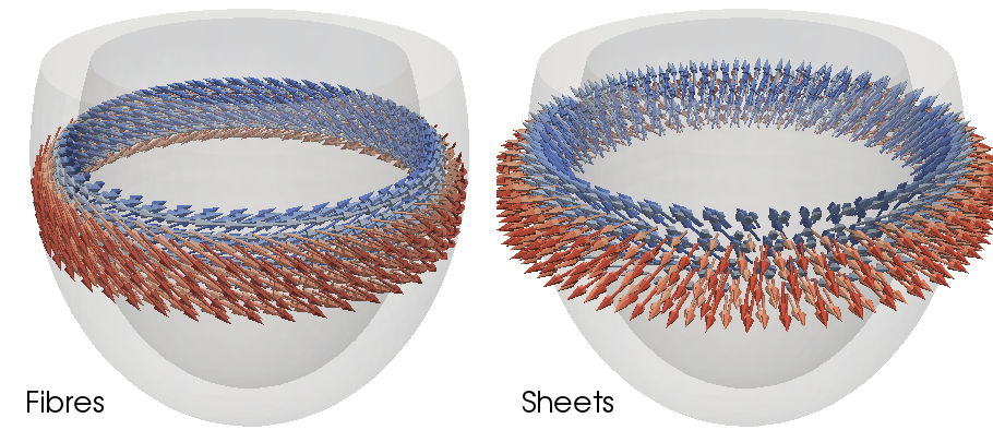
For an accurate simulation of either cardiac electrophysiology or cardiac mechanics, we need to describe the orthotropy of the tissue. In CARP, this is done by setting either just the longitudinal direction of the cardiac myocytes (in the case where we assume that the tissue is isotropic in the transverse directions) or both the longitudinal (“fibre”) direction and the second principal (“sheet”) direction (allowing a fully orthotropic material to be specified).
These fibre orientations are defined on the CARP finite element mesh on a per-element basis with a .lon file. This simple text file has the format:
1
f1_x f1_y f1_z
f2_x f2_y f2_z
...
fn_x fn_y fn_z
or:
2
f1_x f1_y f1_z s1_x s1_y s1_z
f2_x f2_y f2_z s2_x s2_y s2_z
...
fn_x fn_y fn_z sn_x sn_y sn_z
That is, the header is simply the number of directions to be specified, then each line has the Cartesian components of the fibre (and optionally sheet) directions for each element in order. The number of entries must match the mesh’s element file.
Generating a fibre field for a new model can be a challenging task. DTMRI has been used with ex vivo DTMRI models to determine model-specific fibre orientations, but it is not yet routinely available for in vivo cases. We therefore rely on a generic, rule-based approach for determining the tissue orthotropy. This tool implements an algorithm published by Bayer et al. to generate a smooth rule-based fibre field in a biventricular mesh.
Algorithm
Fibre rules are specified by defining the  and
and  angles on the endocardium and epicardium. The fibre orientations are then
interpolated by the algorithm across the wall. The angles determine the fibre
orientations as defined by
Bayer et al. in their paper:
angles on the endocardium and epicardium. The fibre orientations are then
interpolated by the algorithm across the wall. The angles determine the fibre
orientations as defined by
Bayer et al. in their paper:
- The longitudinal fibre direction rotates clockwise throughout the ventricular
walls from the endocardium (
 ) to the epicardium
(
) to the epicardium
( ), where : is the helical angle with resect to
the anticlockwise circumferential direction in the heart with looking from the
base towards the apex.
), where : is the helical angle with resect to
the anticlockwise circumferential direction in the heart with looking from the
base towards the apex. - The transverse fibre direction (sheet direction) is perpendicular to the
longitudinal direction and is defined by the angle :, where
: is the angle with respect to the outward transmural axis of the
heart.
These angles are illustrated in Figure 1 of the above paper.
Both the biventricular and single-ventricle modes of GlRuleFibres use solutions
of Laplace’s equation to determine a “material coordinate system” of sorts. For
example, setting the boundary conditions of  at the apex and
 at the base will result in a smooth 0 to 1 field from apex to
base, which allows you to determine both a normalized distance along this
direction and the local apex-base direction, from the gradient of the Laplace
solution. Multiple such solutions can provide both the knowledge of the position
within the heart (for iterpolation of fibre rules) and a set of local material
axes (providing a basis for the calculation of the fibre direction).
at the base will result in a smooth 0 to 1 field from apex to
base, which allows you to determine both a normalized distance along this
direction and the local apex-base direction, from the gradient of the Laplace
solution. Multiple such solutions can provide both the knowledge of the position
within the heart (for iterpolation of fibre rules) and a set of local material
axes (providing a basis for the calculation of the fibre direction).
Single Ventricle
The single ventricle (or ‘lv’) mode of GlRuleFibers requires only two solutions to Laplace’s equation - an apical-basal solution and a transmural (endocardium to epicardium solution). These are determined by solving Laplace’s equation with the boundary conditions:
| Apical-Basal |
|
| Endo-Epi |
|
The single ventricle mode uses the endo-epi solution to interpolate the fibre angles linearlly across the heart wall, then uses the gradient of both solutions to calculate a basis for determining the fibre orientations from these angles. Note that this works differently from the biventricular mode, which follows the slightly different algorithm in Bayer’s paper.
Biventricular
The biventricular mode of GlRuleFibres follows the inputs and algorithm set out by Bayer et al.. In addition to the solutions to Laplace’s equations needed for the single ventricle case above, additional solutions are needed for the separate ventricles:
| Apical-Basal |
|
| Endo-Epi |
|
| LV |
|
| RV |
|
These required soltuions are illustrated in Figure 2 of the paper of Bayer et al..
The algorithm is explained in full in the above paper, but briefly, the gradients to the above solutions are used to determine the fibre orientation on the LV and RV endocardium and on the epicardium, and the solution values are then used as weights in an interpolation algorithm. The interpolation treats the orientations as quaternions, in order to ensure that the interpolation is smooth in both the longitudinal and transverse directions.
Usage
This script provides a convenient interface to automatically perform all the required solutions to Laplace’s equation and run the fibre generation tool.
Example Mesh
When given no inputs, the tool will automatically generate a mesh of a truncated ellipsoidal shell and apply the single ventricle fibre algorithm to it. Add the –vtk option to generate a VTK mesh including the generated fibre orientations and the computed solutions to Laplace’s equation, providing convenient visualisation in Paraview:
./run.py --vtk
Existing Mesh
To run this script with your own mesh you need:
- A CARP format mesh
- .vtx (vertex) files defining the boundary conditions neeeded:
- Single ventricle: apex, base, endocardium, epicardium
- Biventricular: apex, base, LV endocardium, RV endocardium, epicardium
Mesh Inputs
Set the mesh basename (the path without .pts/.elem etc.) with the –basename option and the mode with the –mode option. The mode can be with ‘lv’ or ‘biv’. The tool will attempt to discover the .vtx file names from the basename, but in the case it cannot find them use the appropriate options in the ‘mesh’ argument group (run ./run.py –help to find these).
Be sure also to set the –myocardium and –non-myocardium options to specify the appropriate element tags for your mesh. This is used to both generate the correct Laplace solutions and to ignore non-myocardium elements in the fibre generation tool. For example, with an LV mesh with myocardial elements with labels 1 and 2 and a cavity with label 10, run:
./run.py --mode lv --basename mymesh --myocardium 1 2 --non-myocardium 10
Fibre Rules
Use the –fibre-rule and –fibre-rule-alpha options to set the fibre rules
you wish to generate. –fibre-rule takes, in degrees,
 ,
,  ,
,
 and
and  , while
–fibre-rule-alpha takes just the angles and uses the
defaults.
, while
–fibre-rule-alpha takes just the angles and uses the
defaults.
You can specify as many fibre rules as you like, of both types above, and the tool will generate a separate .lon file for each. If used with the –vtk option, all fibre fields will be included in the generated .vtk file:
./run.py --mode biv --basename mybivmesh \
        --fibre-rule 40 -50 -65 25       \
        --fibre-rule-alpha 60 -60        \
        --fibre-rule-alpha 75 -75        \
        --vtk