Law of Hagen-Poiseuille
Module: tutorials.06_fluid.01_HagenPouseille_Stationary.run
Section author: Elias Karabelas <elias.karabelas@medunigraz.at>
This example demonstrates a simple application for fluid dynamics in a straight cylindrical pipe.
Law of Hagen-Poiseuille
The law of Hagen-Poiseuille is a physical law that gives the
pressure drop  for an incompressible Newtonian fluid in the laminar regime flowing through a long cylindrical pipe of constant cross section. This geometric
setup is depicted in figure Fig. 166.
for an incompressible Newtonian fluid in the laminar regime flowing through a long cylindrical pipe of constant cross section. This geometric
setup is depicted in figure Fig. 166.
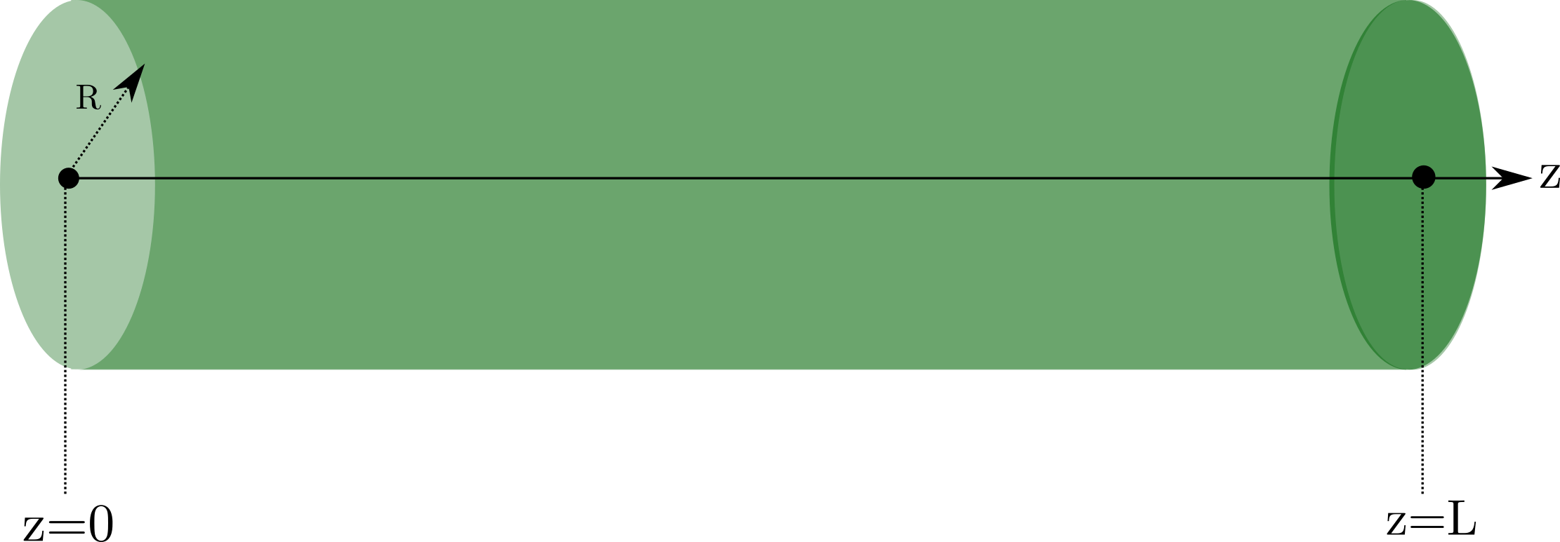
Fig. 166 Geometry for the Hagen-Poiseuille law.
The law states that

where
- is the pressure drop (in Pascal)
 is the length of the pipe (in meter)
 is the dynamic viscosity of the fluid (in Pascal seconds)
 is the volumetric flow rate (in cubic meter per seconds)
 is the pipe radius (in meter)
Derivation of Hagen-Poiseuille’s Law
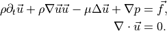
For the derivation we will use the Navier-Stokes equations
First we assume that  and
and  constant. To derive Hagen-Poiseuille’s law we will rewrite the Navier-Stokes
equations in cylindrical coordinates
constant. To derive Hagen-Poiseuille’s law we will rewrite the Navier-Stokes
equations in cylindrical coordinates
(65)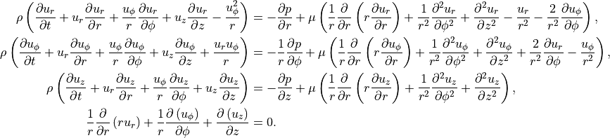
Additionally the following is assumed
- Steady flow, meaning

- Radial and swirl components of the fluid velocity are zero meaning

- The flow is assumed to be axisymmetric, meaning

- The flow is fully developed, meaning

First with this assumptions the continuity equation (fourth line of (65)) is trivially fulfilled. Further it follows that
(66)
From this we can deduce that  . Plugging this into the last line of (66) we can solve for
 by twice integrating and get
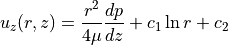
with some arbitrary integration constants  . To get a closed representation we will use the following
observations
. To get a closed representation we will use the following
observations
- On the boundary of the cylinder (
 ) we want
- For
 we want to be finite
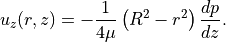
The first obervation yields  and the second yields that
  . Putting all
together we get a closed expression for
. Putting all
together we get a closed expression for
As a last assumption, let $p$ be decreasing linearly from  to
to  yielding
  . Now we can calculate the volumetric flux through the cross section of the cylinder as
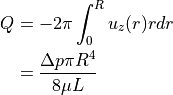
which gives the Law of Hagen-Poiseuille.
Numeric Verification
For the experiments we choose a cylindrical pipe with  . We will vary the pressure drop
as well as the viscosity . For simplicity we assume that
. We will vary the pressure drop
as well as the viscosity . For simplicity we assume that  . We have three
different discretizations (coarse, medium, fine). The coarse discretization has a maximal edge length of
. We have three
different discretizations (coarse, medium, fine). The coarse discretization has a maximal edge length of
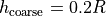 , the medium has
  , and the fine has
 .
.
| [Pa] |
[Pa s] |
 |
|
|---|---|---|---|
| Experiment 1 | 1.0 | 0.01 | 0.625 |
| Experiment 2 | 5.0 | 0.01 | 3.125 |
| Experiment 3 | 10.0 | 0.01 | 6.25 |
| Experiment 4 | 15.0 | 0.01 | 9.38 |
| Experiment 5 | 1.0 | 0.001 | 62.5 |
| Experiment 6 | 5.0 | 0.001 | 312.5 |
| Experiment 7 | 10.0 | 0.001 | 625.0 |
| Experiment 8 | 15.0 | 0.001 | 937.5 |
The results for the coarse discretization are depicted in Table Tab. 22, the results for the
medium discretization are depicted in Table Tab. 23, and the results for the fine discretization
are depcited in Table Tab. 24. One can clearly see the influence of the Reynolds number on the
accuracy of the numeric solution. For  in a cylindrical pipe the assumptions for the law
of Hagen-Poiseuille are not longer valid.
in a cylindrical pipe the assumptions for the law
of Hagen-Poiseuille are not longer valid.
Usage
To run your own validation experiment just type in the command
./run.py --discretization TYPE --mu VALM --rho VALR --pressureDrop VALP --np NP
Here TYPE can be either coarse, medium or fine. This relates to the meshes used. The value VALM is the
value for the dynamic viscosity of the fluid in Pascal seconds. Value VALR is the value for the fluid
density in kilogram per cubic meters. VALP denotes the value for the pressure drop
given in Pascal. At the inflow a value of  will be prescribed and at the outflow a value of
 . Last, NP stands for the number of processors.
The above code uses the standard meshes provided with this run script. This cylindrical mesh has the default length
![L=0.5[m]](../../_images/math/5baaa5baa66a6d8b0ac0d5f2b3dfe91ecc156b45.png) , and default radius
, and default radius ![R=5[cm]](../../_images/math/6927ac731c0bfb9f7c65af1b4ab8a41980ce7dc4.png) . You can also generate your own mesh. This is achieved via the
flags:
. You can also generate your own mesh. This is achieved via the
flags:
./run.py --discretization TYPE --mu VALM --rho VALR --pressureDrop VALP --np NP --generate 1 --radius R --length L
--radiusfactor HR
Here, R denotes the radius of your cylinder in centimeter, L denotes the length of your cylinder in meter and
HR gives the factor for calculating the average edgelength in the mesh. It should be between zero and one. The edgelength is calculated as
 . To use this functionalty you need to have meshtool in your search path as well as gmsh.
The software package gmsh can be downloaded from here. Depending on the chosen parameters the
generation of the meshes can take some time.
. To use this functionalty you need to have meshtool in your search path as well as gmsh.
The software package gmsh can be downloaded from here. Depending on the chosen parameters the
generation of the meshes can take some time.
Coarse
 |
 |
 |
|
|---|---|---|---|
| coarse (1) | 4.8157e-04 | 4.9087e-04 | 0.0190 |
| coarse (2) | 2.4077e-03 | 2.4544e-03 | 0.0190 |
| coarse (3) | 4.8157e-03 | 4.9087e-03 | 0.0190 |
| coarse (4) | 7.2243e-03 | 7.3631e-03 | 0.0188 |
| coarse (5) | 4.5198e-03 | 4.9087e-03 | 0.0792 |
| coarse (6) | 2.0044e-02 | 2.4544e-02 | 0.1833 |
| coarse (7) | 3.6429e-02 | 4.9087e-02 | 0.2579 |
| coarse (8) | 5.0822e-02 | 7.3631e-02 | 0.3098 |
Medium
|
|
|
|
|---|---|---|---|
| medium (1) | 4.8869e-04 | 4.9087e-04 | 0.0044 |
| medium (2) | 2.4435e-03 | 2.4544e-03 | 0.0044 |
| medium (3) | 4.8875e-03 | 4.9087e-03 | 0.0043 |
| medium (4) | 7.3321e-03 | 7.3631e-03 | 0.0043 |
| medium (5) | 4.8394e-03 | 4.9087e-03 | 0.0141 |
| medium (6) | 2.3317e-02 | 2.4544e-02 | 0.05 |
| medium (7) | 4.5841e-02 | 4.9087e-02 | 0.0661 |
| medium (8) | 6.7741e-02 | 7.3631e-02 | 0.08 |
Fine
|
|
|
|
|---|---|---|---|
| fine (1) | 4.9044e-04 | 4.9087e-04 | 0.0009 |
| fine (2) | 2.4523e-03 | 2.4544e-03 | 0.0009 |
| fine (3) | 4.9046e-03 | 4.9087e-03 | 0.0008 |
| fine (4) | 7.3573e-03 | 7.3631e-03 | 0.0008 |
| fine (5) | 4.9081e-03 | 4.9087e-03 | 0.0001 |
| fine (6) | 2.3535e-02 | 2.4544e-02 | 0.0411 |
| fine (7) | 4.6091e-02 | 4.9087e-02 | 0.0610 |
| fine (8) | 6.9728e-02 | 7.3631e-02 | 0.0530 |