`Optical mapping`

Module: tutorials.02_EP_tissue.10_optical.run

Section author: Martin Bishop <martin.bishop@kcl.ac.uk

Optical Mapping Post-Processing

Optical mapping is an experimental technique that utilises fluorescent voltage-sensitive dyes to record changes in transmembrane potential from the surface of cardiac tissue. The fundamental basic principles of fluorescent voltage-sensitive imaging are described below. More details on optical mapping are found in the CARPentry manual.

Basics of Fluorescent Voltage-Sensitive Imaging

Optical mapping is an experimental technique that utilises fluorescent voltage-sensitive dyes to record changes in transmembrane potential from the surface of cardiac tissue. A change in the intensity of the recorded voltage-sensitive fluorescent emission must be related back to the change in membrane potential at the cellular level. As a result, standard optical mapping techniques cannot be used to measure absolute transmembrane potential levels, but instead can merely track changes in membrane potential. Common experimental practice is to normalise the fluorescent signal on a pixel by pixel basis with respect to the AP maximum and minimum values obtained following a pacing protocol. This procedure also addresses the potential problem of variations in the intensity and spatial distributions of the dye staining throughout the preparation which can affect the local intensity of the recorded fluorescence.

The basic setup of an optical mapping experiment in CARPentry is shown in Fig. 14.

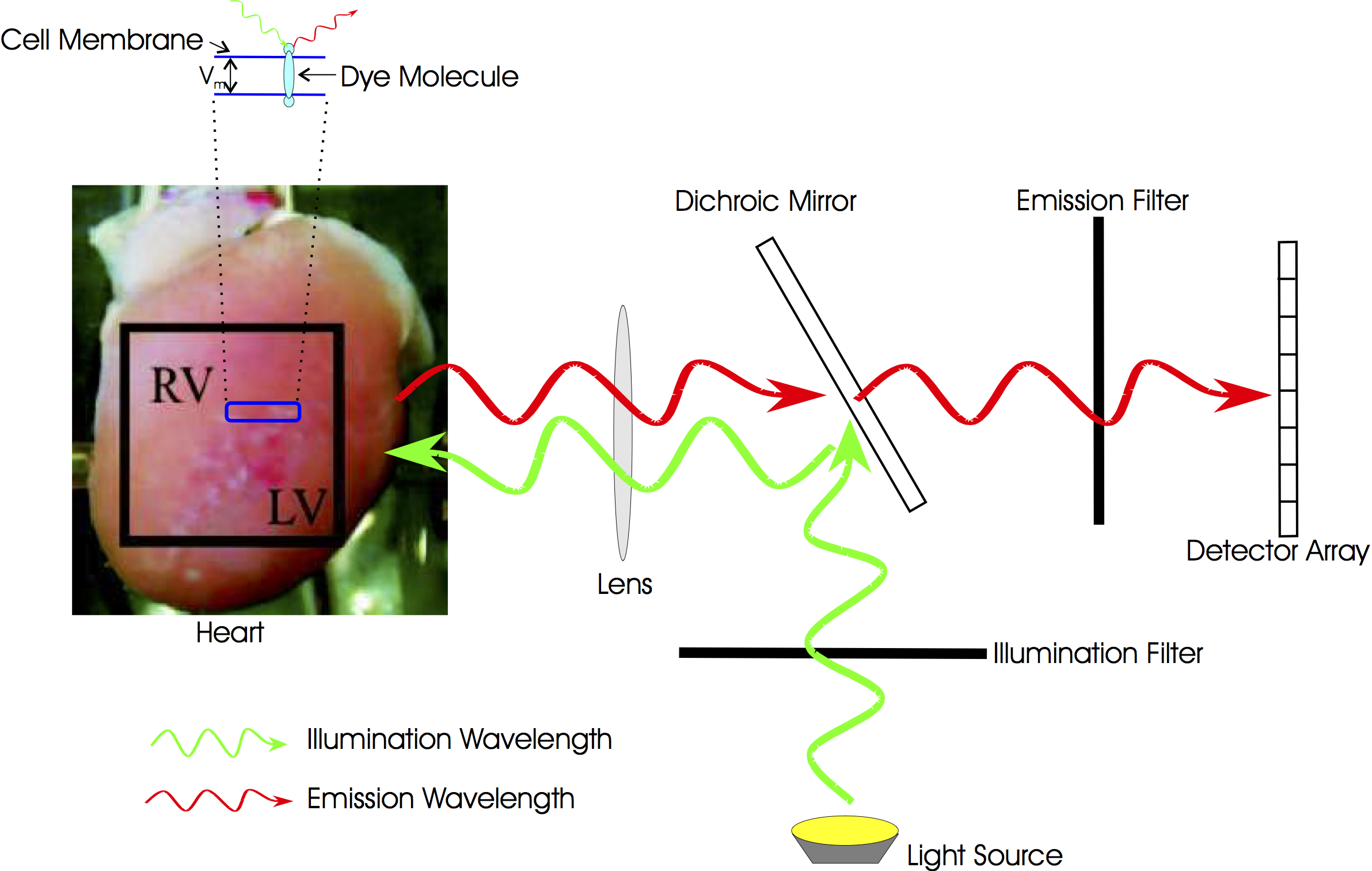
Fig. 112 Typical optical mapping setup in CARPentry showing the boundary conditions imposed for illumination and fluorescent emission.

Note that optical mapping post-processing option computes the simulated optical signal based on a previously computed voltage file as input along with the corresponding mesh.

Simulating Optical Mapping Signals

Simulating the signals obtained by optical mapping recordings requires the simulation of light (photon) propagation through cardiac tissue. Cardiac tissue, like most biological tissue, is highly scattering and relatively weakly absorbing to light at the wavelengths commonly used in experimental fluorescent imaging. In such cases, the movement of photons throughout the tissue can be modelled mathematically using either a continuous (reaction-diffusion) or a discrete (stochastic) approach. CARPentry uses the latter approach.

The continuum approximation to the simulation of photon transport within biological tissue does not consider the movement of individual photons, but instead they are considered to move as one continuous entity, which causes a resulting change in spatially distributed properties associated with the tissue as a whole as they move. For example, this allows us to write-down differential equations which represent the change in space and time of the photon density throughout the tissue, as the photons diffuse and scatter within the medium. The situation is directly analogous to the classic reaction-diffusion style heat equation, where the spread of heat along a material is modelled, which in fact arises due to individual vibrations at the atomic level.

The Photon Diffusion Equation

The steady-state form of the photon diffusion equation is considered as the time-scales involved in changes in electrical activation are many orders of magnitude larger than the time-scales involved in photons reaching equilibrium within the tissue. The steady-state photon diffusion equation for highly scattering media is therefore given by

$D \nabla^2 \Phi - \mu_a \Phi = -w$

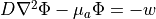
where $\Phi$ is the photon density within the tissue, $D$ is the diffusivity, $\mu_a$ is the absorption coefficient and $w$ is the source of photons. The optical properties take on differernt values at the illumination wavelength (usually 500 nm or so) and emission wavelengths (usually 600 nm or so). Typical values are $D^{illum}=0.19$ mm, $D^{em}=0.36$ mm, $\mu_{a}^{illum}=0.52mm^{-1}$ and $\mu_{a}^{em}=0.12mm^{-1}$ .

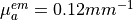Process of Simulating an Optical Mapping Signal

Simulation of an optical signal is a multi-stage process. Firstly, the raw transmembrane potential signal is simulated in CARPentry for the particular protocol of interest. This is the “true” activity within the tissue and acts as an input to the model. The other input is the illuminating photon density, $\Phi_{illum}$ . The value of $V_{m}$ and $\Phi_{illum}$ are then combined at every node in the mesh to represent the source of fluorescent emission - this represents the physical situation as the larger the $V_{m}$ value, the larger the fluorescent emission from a point, and the more illuminating light that point receives, then the larger the emission from that site. Once the photon density at the emission wavelength throughout the tissue is found $\Phi_{em}$ , we are interested in the flux of photon density exiting the tissue surface. Thus, we apply Fick’s Law to obtain this flux, which represents the photons exiting from the tissue surface to be collected. Note that we usually assume that we are simulating an epi-fluorescent setup whereby the illuminating and detection surface are the same. This process is summarised in Fig. 15 and each step described in more detail below.

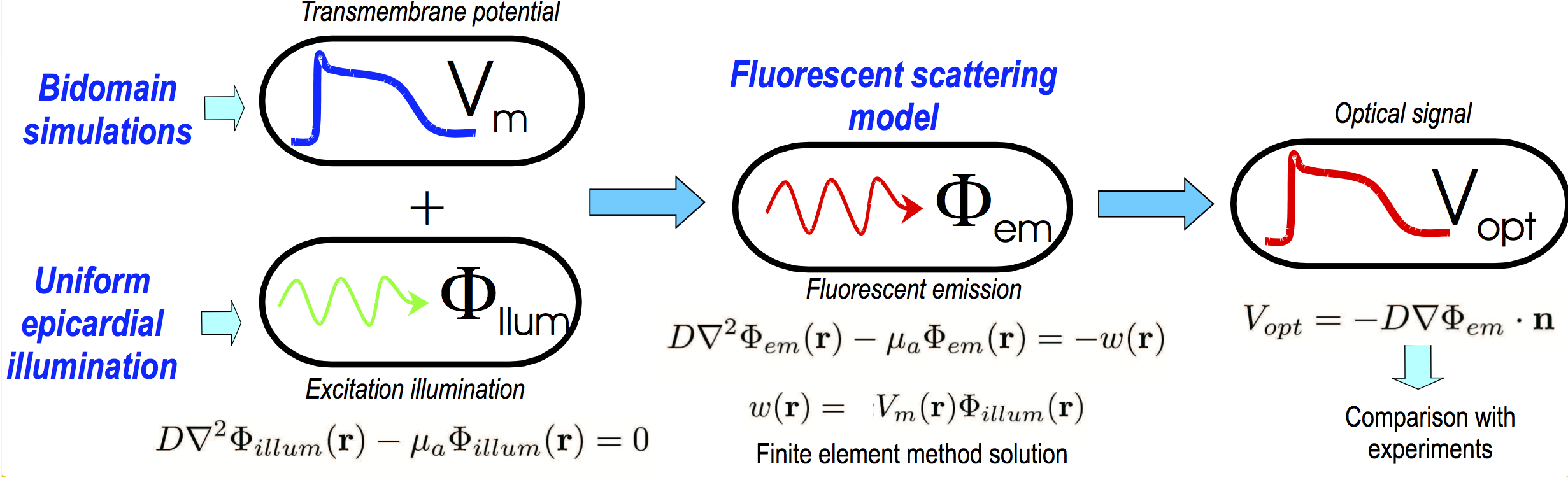
Fig. 113 Schematic process by which optical mapping signals are simulated in CARPentry.

Simulating Illumination

During illumination, we need to define a surface which we choose to illuminate. The is usually the epicardium. No souces of illumination light exist within the tissue here, so $w=0$ . The analytic solution to the illumination problems gives a simple exponential decay into the tissue, decaying fro the epicardial surface. The value of the illumination at the surface is irrelevant as only the relative decay (or the profile) of the illuminating light into the tissue is important (i.e. all optical mapping signals are normalised).

Simulating Fluorescent Emission

The emission problem solves the same equation, but here we do have sources of (fluorescent) photons within the tissue so $w \neq 0$ . The source of fluorescence is modelled as

$w = \Phi_{illum} V_{m}$

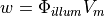
where $\Phi_{illum}$ represents the density of photons due to the illuminating light and $V_{m}$ is simply the value of the transmembrane potential. Note that because, physically, we can never have a negative source of photons, $w$ always has to be positive. Therefore, $V_{m}$ must always be positive and so we normalise it to the amplitude of an action potential (-80-40 mV). To account for very negative values of $V_{m}$ during shocks, we further choose to normalise such at a normal AP goes between $9-10$ to avoid $V_{m}$ ever being negative. This also is physical, as it represents real experiments, in which only a fractional change in $V_{m}$ is observed on a background of fluorescence. Once $\Phi_{em}$ is found, we compute the gradient of it at the surface using Fick’s law to obtain the simulated optical signal

$V_{opt} = -D \Phi_{em} \cdot \hat{\mathbf{n}}$

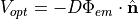
where here we make the assumption that all of this signal is collected.

Boundary Conditions

Like in the bidomain, on any surfaces which don’t have a specific illumination or emission boundary condition imposed we assume the standard zero flux condition of $\Phi = 0$ . This is ok for the sides of a slab, for example, which is being illuminated from its top side. However, for the base of the slab this isn’t adequate, and additional boundary conditions during both illumination and emission should be specified here. Specifically, $\Phi=0$ should be defined on these surfaces. This should only be worried about for thin slabs. For anything thicker than approximatley 2 mm or so, it doesn’t really matter, as the illuminating photon density will have decayed to almost zero here anyway (although this should be adjusted for different illuminating wavelengths which may penetrate deeper, as appropriate).

It is important to note that all real-life optical mapping signals will be distorted at the boundaries of the tissue (i.e. the edges of a wedge preparation etc) and so given the non-ideal nature of the boundary conditions applied at the sides of a wedge, the signals in this vicinity (as in an experiment) should not be used. Furthermore, the vast majority of optical imaging of this nature will take place on tissue that is >1 mm thick, and so imposing a zero Dirichlet boundary condition on the lower surface (furthest away from the illuminated surface) is a reasonable approximation.

A schematic representation of the necessary boundary conditions are shown below in Fig. 16.

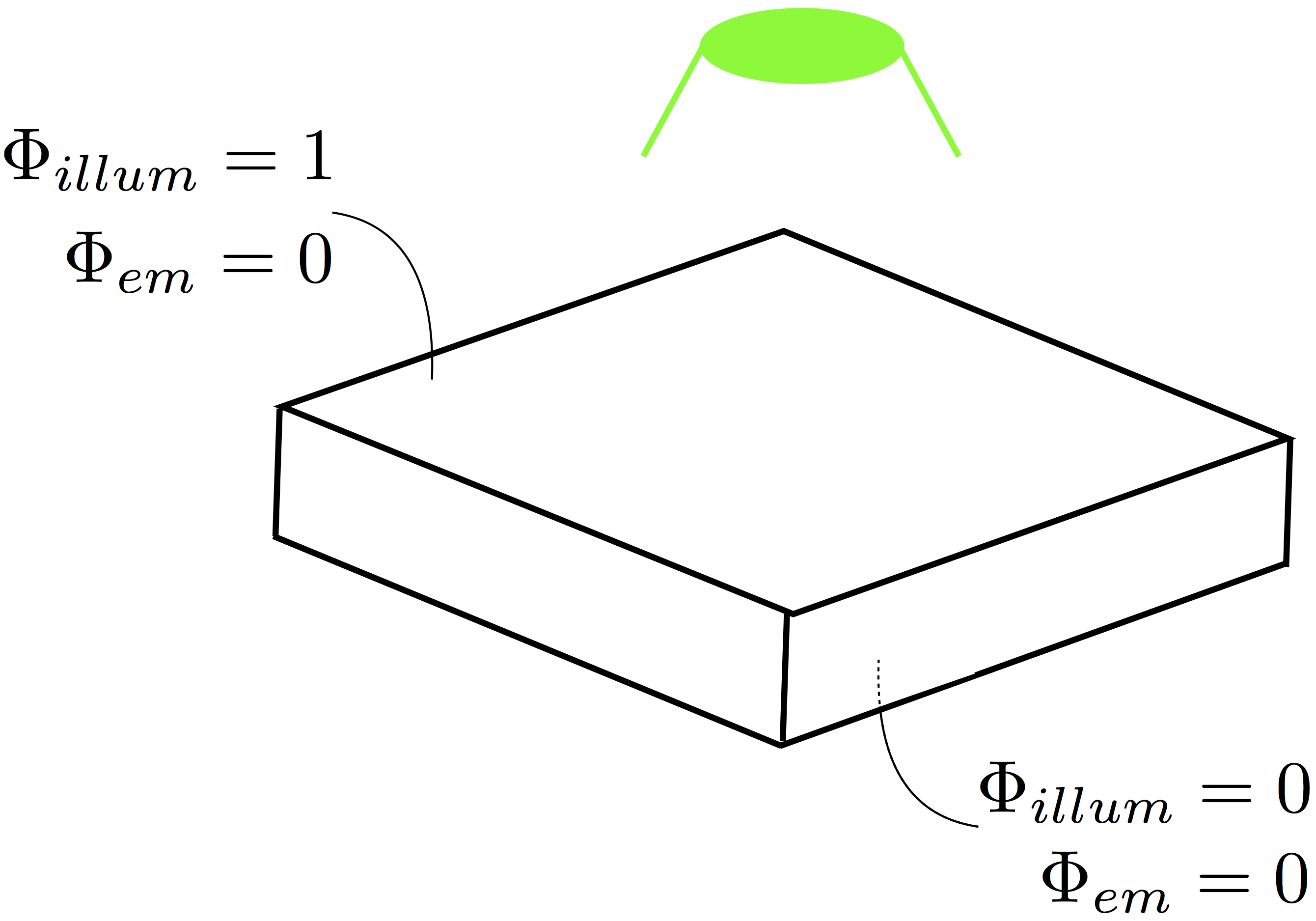
Fig. 114 Typical boundary conditions applied to a tissue setup for an optical mapping simulation.

Practical Implementation in CARPentry

Optical mapping is run as a post-processing option as it requires the pre-computation of $V_{m}$ . It is run with -post_processing_opts 2 and outputs files in the POSTPROC_DIR as with any other post-processing simulation. To run an optical mapping experiment, both illuminating and emitting (or recording) surfaces need to be defined. These are setup and defined like stimulating electrodes, being termed illum_dbc and emission_dbc as they represent Dirichlet boundary conditions thus having a bctype of 1.

Like electrodes, they can be defined as a collection of points with boxes or with a list of vertices. However, note that these points must lie on the surface of the tissue that you want to illuminate. The illum_dbc.strength parameter should just be set to 1, although the magnitude doesn’t really matter (all magnitudes are relative in optical mapping). Example illumination boundary conditions may be as follows:

# defines illuminated surface first (epicardium)
illum_dbc[0].bctype     =     1
illum_dbc[0].x0         =  -2000
illum_dbc[0].xd         =   4000
illum_dbc[0].y0         = -2000
illum_dbc[0].yd         =  4000
illum_dbc[0].z0         = 900
illum_dbc[0].zd         = 200
illum_dbc[0].strength   =   1

# defines endocardium where we fix Phi to be 0
illum_dbc[1].bctype     =     1
illum_dbc[1].x0         =  -2000
illum_dbc[1].xd         =   4000
illum_dbc[1].y0         = -2000
illum_dbc[1].yd         =  4000
illum_dbc[1].z0         = -1100
illum_dbc[1].zd         = 200
illum_dbc[1].strength   =   0

For now the em_dbc.strength is set to 0 on the surfaces from which you would like to compute the signal. This is the most natural choice as described above. We assume that exactly just outside the tissue, there is no scattering, so photons rapidly move-off to infinity, thus leaving zero photon density just the other side of the boundary. There is a more accurate mixed Neumann/Diricthlet boundary condition that could be implemented here, but the differences are minimal (less than <5 % between this and the more simple case of $\Phi_{em}=0$ ). Example emission boundary conditions may be as follows:

# bcs for 0 Dirichlet bc on upper illuminated surface (epicardium)
emission_dbc[0].bctype     =     1
emission_dbc[0].x0         =  -2000
emission_dbc[0].xd         =  4000
emission_dbc[0].y0         = -2000
emission_dbc[0].yd         =  4000
emission_dbc[0].z0         = 900
emission_dbc[0].zd         = 100
emission_dbc[0].strength   =     0

# Additional bcs for 0 Dirichlet bc on lower surface (endocardium)
emission_dbc[1].bctype     =     1
emission_dbc[1].x0         =  -2000
emission_dbc[1].xd         =  4000
emission_dbc[1].y0         = -2000
emission_dbc[1].yd         =  4000
emission_dbc[1].z0         = 900
emission_dbc[1].zd         = 100
emission_dbc[1].strength   =     0

Experimental Parameters

The main parameters considered in this tutorial relate to the optical parameters which govern the optical properties of the tissue. The optical parameters which describe the optical absorption and scattering properties of the tissue at both the illumination and emission wavelengths are given by mu_a_illum, mu_a_em, Dopt_illum and Dopt_em. Values for these can be found in Bishop et al (2006) [1].

Changing the illumination parameters affect how easily light gets into the tissue; changing the emission parameters alters how easily light exists the tissue.

Output

The outputs from this function are igb files defining phi_illum, w and Vopt. The main ouput is obviously Vopt and can be loaded-up into Meshalyzer. Note, however, that if trying to view the source term w, then due to the boundary conditions described above, it will appear 0 on all specified emission boundaries (i.e. on the external surfaces). Applying a clipping plane through the tissue will, however, expose the functional form of w.

Prior to normalisation, the raw output of Vopt may look a bit strange and patchy. It is up to the user to compute a normalised version of Vopt in which every node is normalised based on the max/min of a paced sinus beat (of a simulated optical action potential). This has been automatically incorporated as part of the below run scripts. The normalised data is saved as normVopt.igb.

Experiments

Several types of optical experiments are predefined. To run these experiments

cd ${TUTORIALS}/02_EP_tissue/10_optical

Run

./run.py --help

to see all exposed experimental parameters.

Experiment exp001

This experiment runs an optical simulation of a single paced beat occurring within the centre of a cuboid mesh.

Run this experiment by

./run.py --visualize

This experiment simply computes the optical signal using the default values of the optical parameters. Note that initially the first Meshalyzer windown to open will be for the vm.igb data. Highlight node 2506 and display the Timeseries data. Note the sharpness of the action potential upstroke.

Once this initial Meshalyzer window is closed, another one opens with the simulated (normalised) optical data normVopt.igb. Click again on the same node and view the Timeseries data. Note the significantly prolonged optical action potential.

It is also possible to load-up the illumination profile into Meshalyzer (contained in phi_illum.igb). Here you can see the charactersitic decay of the illuminating light through the tissue.

Experiment exp002

This experiment repeats the first one above, but this time alters both the illumination and emission absorption properties of the tissue.

Run this experiment by

./run.py --mua_illum 0.88 --mua_em 0.16 --visualize

which simulates the effect of tissue which heavily absorbs light (or operates at a shorter wavelength).

Repeat the experiment by

./run.py --mua_illum 0.07 --mua_em 0.05 --visualize

Which simulates the effect of tissue which lightly absorbs light (or operates at a longer wavelength).

These parameters are as obtained from Walton et al (2010) [2].

Literature

[1]	Bishop et al, Synthesis of Voltage-Sensitive Optical Signals: Application to Panoramic Optical Mapping, Biophysical Journal, 90(8):2938-2945, 2006. [PubMed] [PMC] [Full]

[2]	Walton et al, Dual excitation wavelength epifluorescence imaging of transmural electrophysiological properties in intact hearts, Heart Rhythm, 7:(12):1843-1849, 2010. [PubMed] [Full]