Electrical Mapping
Module: tutorials.02_EP_tissue.08_lats.run
Section author: Fernando Campos <fernando.campos@kcl.ac.uk>
This tutorial demonstrates how to compute local activation times (LATs) and action potential durations (APDs) of cells in a cardiac tissue.
Electrical Mapping
The wavelength of the cardiac impulse, given by the product of conduction velocity (CV) and refractory
period, is of utmost importance for the study of arrhythmia mechanisms. The assessment of the CV as
well as the refractory period of the cardiac action potential (AP) relies on the determination of
activation and repolarization times, respectively. Experimentally, these are usually calculated based
on 1) transmembrane voltages  measured by glass micro-electrodes or in optical
mapping; or 2) extracellular potentials
measured by glass micro-electrodes or in optical
mapping; or 2) extracellular potentials  measured at the surface of the tissue.
The estimation of activation/repolarization times is based on an event detector that records the
instants when the selected event type occurs. Local activation time (LAT), for instance, is usually
taken as the time of maximum  or the minimum
  :
:
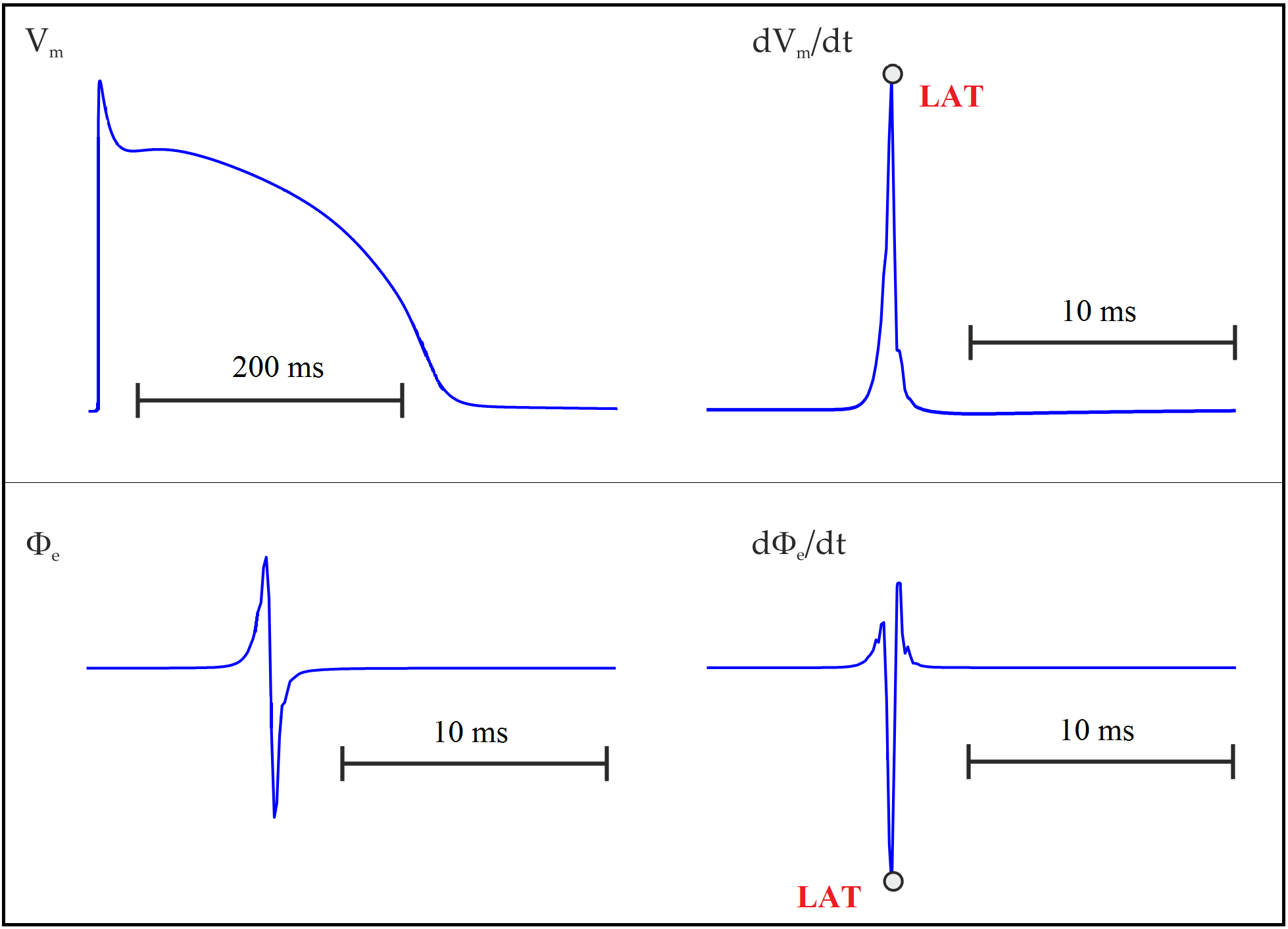
Fig. 106 Action potential in an uncoupled cell. Upper panel: transmembrane potential
and its time derivative . Lower panel: extracellular potential
and its time derivative . LAT is usually taken as the time of maximum
or the minimum .
Instead of using derivatives, LATs can also been estimated by the crossing of a threshold value provided
that the chosen value reflects the sodium channel activation since they are responsible for the rising
phase of AP. One could, for instance, pick the time instant when crosses -10 mV
with a positive slope. Equally, one could look for crossing of with a negative
slope to detect repolarization events. AP duration (APD) can then be computed as the difference between
repolarization and activation times. The detection of activation ( ) and repolarization
(
) and repolarization
( ) times based on threshold crossing is illustrated below:
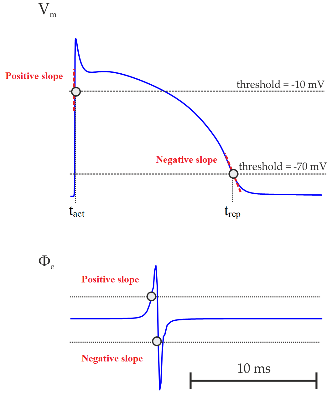
Fig. 107 Activation (LAT) and repolarization times and
computed using the threshold crossing method. 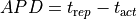 .
.
Problem Setup
This example will run a simulation using a 2D sheet model (1 cm x 1 cm). A transmembrane stimulus
current of 100 uA/cm^2 is applied for a period of 1 ms at the middle of the left side of the tissue.
A ground electrode is placed at the opposite side of the stimulating electrode. Simulation of electrical
activity is based on the bidomain equations. Cellular dynamics cardiac myocytes within the tissue are
described using the Modified Beeler-Router Drouhard-Roberge (MBRDR) model. Activation times are obtained
either from or using a threshold crossing method, whereas
repolarization can only be obtained by threshold crossing from . Estimation of
repolarization times from is out of the scope of this tutorial.
Usage
To run this tutorial :
cd tutorials/08_lats

./run.py --help
The following optional arguments are available (default values are indicated):
--quantity          Quantity/variable/signal used to compute activation time
                    Options: {vm,phie}
                    Default: vm
--act-threshold     The threshold value for determining activation from :math:`V_{\mathrm m}` or :math:`\phi_{\mathrm e}`
                    Default: -10 mV
--rep-threshold     The threshold value for determining repolarization from :math:`V_{\mathrm m}
                    Default: -70 mV
--show-APDs         Visualize APDs instead of LATs
If the program is run with the --visualize option, meshalyzer will automatically load the computed
activation sequence (LATs). If the --show_APDs is given, then the computed APDs will be loaded:
Visualize LATs:
./run.py --visualize

Visualize APDs:
./run.py --show-APDs
Interpreting Results
Differences between activation sequences computed from or
and/or with different thresholds can be appreciated with meshalyzer (--visualize). The activation
sequence for the default parameters looks like this:
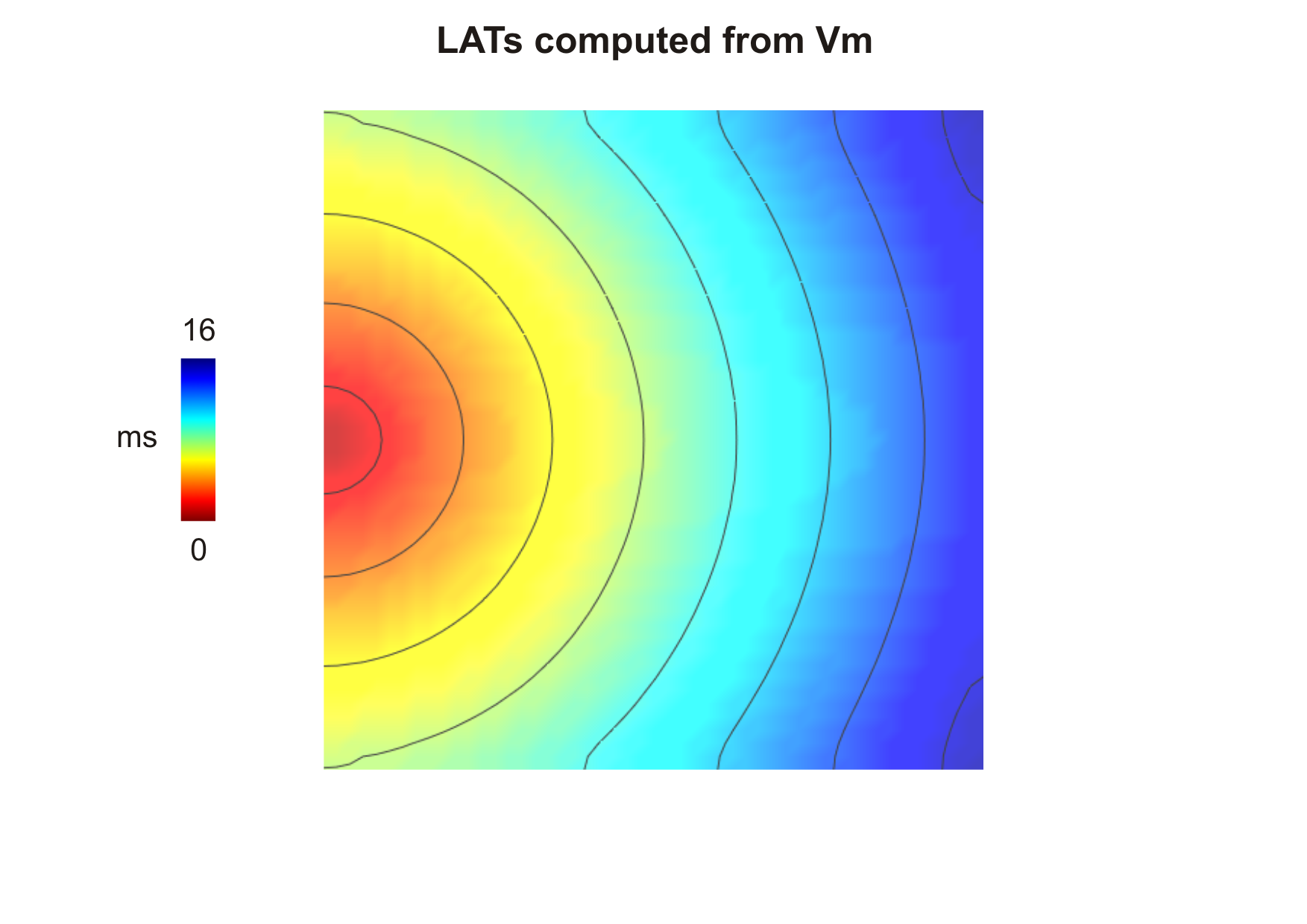
Fig. 108 Activation sequence computed from (--act-threshold=-10) obtained after
delivering a stimulus current in the middle of the left side tissue.
Note
- It is important to note that while computing activation from -lats[].mode
has to be set to zero. This is because is about -85 mV in cardiac cells
at rest and rapidly rises to about +40 mV during the activation phase. This means
will cross the threshold with a positive slope. While computing repolarization, on the other
hand, goes from positive values back to the rest. The threshold will be
then crossed with a negative slope.
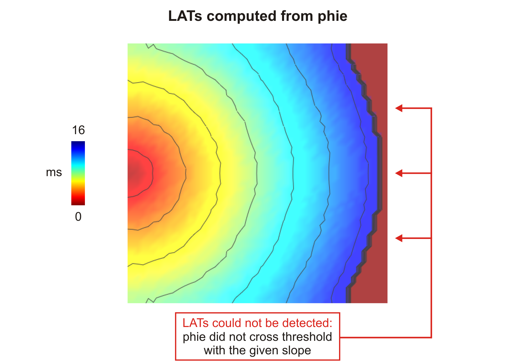
Fig. 109 Activation sequence computed from (--act-threshold=-10) obtained
after delivering a stimulus current in the middle of the left side tissue.
Note
- Unlike the shape of which remains pretty much the same in all cells,
morphology may vary depending on its position in relation to both
stimulation and ground electrodes. Thus, LATs obtained based on
might differ from those obtained from .
- If the criteria for threshold crossing detection is never satisfied, the resulting entry in
the output file will be -1. See action sequence obtained from .
The computed APDs using the default parameters looks like this (use --show-APDs instead of --visualize):
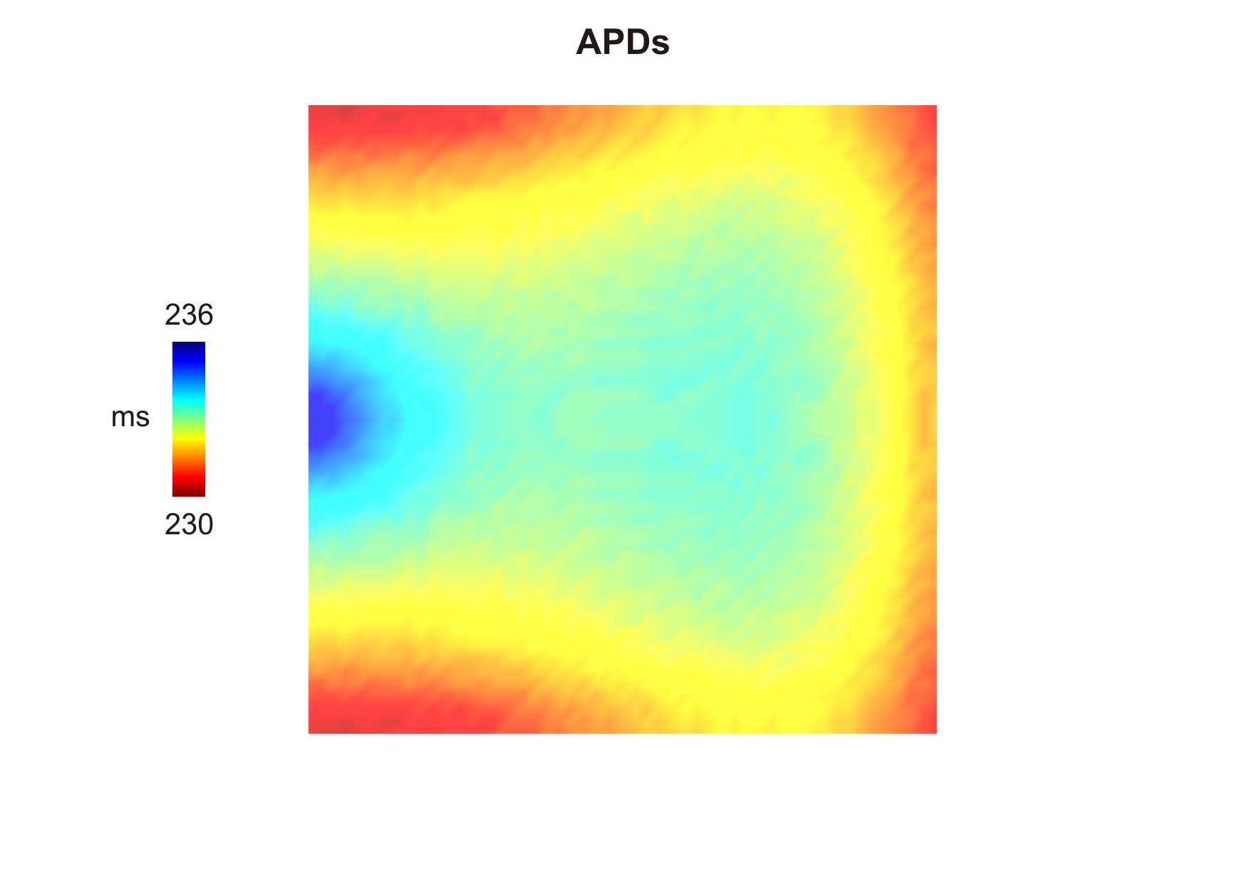
Fig. 110 Action potential durations computed using the default thresholds (--act-threshold=-10 and
--rep-threshold=-70) after delivering a stimulus current in the middle of the left side of
the tissue.
CARPentry Parameters
The relevant parameters used in the tissue-scale simulation are shown below:
# Number of events to detect
-num_LATs  = 2

# Event 1: activation
-lats[0].ID         = 'ACTs'
-lats[0].all        = 0
-lats[0].measurand  = 0
-lats[0].threshold  = -10
-lats[0].mode       = 0

# Event 2: repolarization
-lats[1].ID         = 'REPs'
-lats[1].all        = 0
-lats[1].measurand  = 0
-lats[1].threshold  = -70
-lats[1].mode       = 1
num_LATs referes to the number of events we want to detect. In this tutorial there are two events:
activation and repolarization. -lats[0] are options to compute activation while -lats[1] are options
to compute repolarization. -lats[].ID is the name of output file; -lats[].all tells CARP if it should
detect only the first event (-lats[].all = 0), i.e. first beat, of all of them (-lats[].all = 1);
-lats[].measurand refers to the quantity: (0) or (1);
-lats[].threshold is the threshold value for determining the event; finally, -lats[].mode tells CARP
to look for threshold crossing with a either a positive or negative slope.