Basic usage of code generation tool limpet_fe.py
Module: tutorials.01_EP_single_cell.04_limpet_fe.run
Section author: Edward Vigmond <edward.vigmond@ubordeaux-1.fr>
This tutorial explains the basics of using the code generation tool limpet_fe.py
for generating ODE solver code for models of cellular dynamics.
A more detailed explanation of the background is found in the section on code generation
in the CME manual.
Usage of limpet_fe.py
limpet_fe.py is the EasyML to C translator for writing ionic models.
The easiest way to see how to write a model is to examine a simpler example.
To work on this tutorial do
cd ${TUTORIALS}/01_EP_single_cell/04_limpet_fe
Input .model file
Let’s look at the
Beeler-Reuter model as modified by Drouhard and Roberge:
Iion; .nodal(); .external();
V; .nodal(); .external(Vm);

V; .lookup(-800, 800, 0.05);
Ca_i; .lookup(0.001, 30, 0.001); .units(uM);

V_init = -86.926861;

# sodium current
GNa = 15;
ENa  = 40.0;
I_Na = GNa*m*m*m*h*(V-ENa);
I_Na  *= sv->j;

a_m = ((V < 100)
       ? 0.9*(V+42.65)/(1.-exp(-0.22*(V+42.65)))
       : 890.94379*exp(.0486479163*(V-100.))/
            (1.+5.93962526*exp(.0486479163*(V-100.)))
       );
b_m = ((V < -85)
       ? 1.437*exp(-.085*(V+39.75))
       : 100./(1.+.48640816*exp(.2597503577*(V+85.)))
       );
a_h = ((V>-90.)
       ? 0.1*exp(-.193*(V+79.65))
       : .737097507-.1422598189*(V+90.)
       );
b_h = 1.7/(1.+exp(-.095*(V+20.5)));

a_d = APDshorten*(0.095*exp(-0.01*(V-5.)))/
  (exp(-0.072*(V-5.))+1.);
b_d = APDshorten*(0.07*exp(-0.017*(V+44.)))/
  (exp(0.05*(V+44.))+1.) ;

a_f = APDshorten*(0.012*exp(-0.008*(V+28.)))/
  (exp(0.15*(V+28.))+1.);
b_f = APDshorten*(0.0065*exp(-0.02*(V+30.)))/
  (exp(-0.2*(V+30.))+1.);

a_X = ((V<400.)
       ? (0.0005*exp(0.083*(V+50.)))/
       (exp(0.057*(V+50.))+1.)
       : 151.7994692*exp(.06546786198*(V-400.))/
       (1.+1.517994692*exp(.06546786198*(V-400.)))
       );

b_X   = (0.0013*exp(-0.06*(V+20.)))/(exp(-0.04*(V+20.))+1.);

xti   = 0.8*(exp(0.04*(V+77.))-1.)/exp(0.04*(V+35.));

I_K = (( V != -23. )
       ? 0.35*(4.*(exp(0.04*(V+85.))-1.)/(exp(0.08*(V+53.))+
                                              exp(0.04*(V+53.)))-
               0.2*(V+23.)/expm1(-0.04*(V+23.)))
       :
       0.35*(4.*(exp(0.04*(V+85.))-1.)/(exp(0.08*(V+53.))+
                                            exp(0.04*(V+53.))) + 0.2/0.04 )
       );

# slow inward
Gsi = 0.09;
Esi = -82.3-13.0287*log(Ca_i/1.e6);
I_si = Gsi*d*f*(V-Esi);
I_X  = X*xti;

Iion= I_Na+I_si+I_X+I_K;

Ca_i_init = 3.e-1;
diff_Ca_i = ((V<200.)
             ? (-1.e-1*I_si+0.07*1.e6*(1.e-7-Ca_i/1.e6))
             : 0
             );

group {
  GNa;
  Gsi;
  APDshorten = 1;
} .param();

group {
  I_Na;
  I_si;
  I_X;
  I_K;
} .trace();
Generally, it looks like C code with a few extra commands. Let’s break it down a bit:
Iion; .nodal(); .external();
V; .nodal(); .external(Vm);
These lines are very important. .external() tells us that these are global variables and through these variables
we will interact with the simulation. The argument to external() is the actual name of the global variable if we want to call it something else locally. Here, the local variable V is actually the global variable Vm while Iion is the
global name which we use locally. To alter the transmembrane voltage, Iion must be assigned a value. CARPentry then uses this value of Iion to adjust the transmembrane voltage.
You do not specify the change *Vm*.
Note
Ionic models are fully functioning models. Plugins are additional components which must be added to an ionic model. They modify or expand behaviour, eg., a new channel or a force genration description. For an ionic model, the ionic current is set, e.g., Iion = 2.3, while plug-ins add an additional current to an existing current, i.e., Iion = Iion + 2.3
The next two lines
V; .lookup(-800, 800, 0.05);
Ca_i; .lookup(0.001, 30, 0.001); .units(uM);
tell the translator to use lookup tables for variables which are functions of these variables in order to avoid expensive function calls. The table range for V is -100 to 100 in steps of 0.05. This should be done after the model is verified to be working correctly.
There are several Hodgkin-Huxley type gating variables. Here is the f gate
a_f = APDshorten*(0.012*exp(-0.008*(V+28.)))/
  (exp(0.15*(V+28.))+1.);
b_f = APDshorten*(0.0065*exp(-0.02*(V+30.)))/
  (exp(-0.2*(V+30.))+1.);
Variables of the form a_XXX and b_XXX are automatically recognized as the  and
and  coefficients. The differential equation for the variable XXX will be automatically generated as well as an intial condition. Alternatively, one can assign tau_XXX and XXX_inf, which correspond to
  and
and  .
.
Note
if a variable is a differential variable but is NOT a recognized gating variable, its initial condition init_XXX must be explicitly set. That is why you will find Ca_i_init in the .model file.
The block:
group {
    GNa;
    Gsi;
    APDshorten = 1;
  } .param();
declares variables with default values. However, their values can be changed at the start of a simulation with the parameter changing syntax.
The section:
group {
  I_Na;
  I_si;
  I_X;
  I_K;
} .trace();
declares a group of trace variables. If a node is selected as being traced, these quantities will be output as functions of time at the node.
Units
Units are a never ending source of grief. All sorts are used in various papers. CARPentry expects certain standards so that interactions are possible between components. The table below gives the recommended units
| quantity | units |
|---|---|
| membrane current | 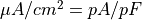 |
| dX/dt |  |
![[Ca]_i](../../_images/math/40a99f21392878df335a167ec57f7b06bda82677.png) |
 |
| [X] |  |
| voltage/potential |  |
| membrane conductance |  |
 |
 |
 |
|
Internally, you can use what you like but you need to convert any variables passed between CARP and your model, i.e., the total membrane current, concentrations, derivatives, and variables associated with gates.
Generating the C source
Once the model file is written, it needs to be converted to C code for compilation
limpet_fe.py my_MBRDR.model
Provided you have no errors, this will produce the files, my_MBRDR.c and my_MBRDR.c. Now, we need to make a runtime shared object library:
make_dynamic_model.sh my_MBRDR
which will produce my_MBRDR.so and which will be accessible as an ionic model with the name my_MBRDR.
Using the IMP
Single cell
The program bench is used to run single cell experiments. See bench for more details running this program. In this tutorial,*run.py* is just a wrapper for bench:
run.py --load-module ./my_MBRDR.so
Note
for the –load option, an absolute path must be specified. That is why we used the “./” in “./my_MBRDR.so”. If the –imp option is not specified, it will attempt to load the ionic model with the same name as the loaded library.
Remembering that we set APDshorten as a parameter, we can see its effect
run.py --load-module ./my_MBRDR.so --imp-par='APDshorten=3'
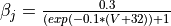
- As an exercise, try adding
Ca_ias a trace variable, or add a J gate to the sodium channel described by the follwing equations 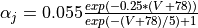 and
and
Parameter files
To use the ionic model in a tissue simulation, it is specified in the parameter file as
num_external_imp = 1
external_imp = ./my_MBRDR.so
imp_region[0].im = my_MBRDR
Obviously, multiple IMPs can be added by increasing num_external_imp.